The first post in this series presented two contrasting approaches for minimizing the average loss \(\frac{1}{n} \sum_{i=1}^n f_i(x)\). One is SGD and variants, whose computational steps amount to choosing \(f \in \{f_1, \dots, f_n\}\) and computing

\[x_{t+1} = \operatorname*{argmin}_x \Biggl\{ \underbrace{\color{blue}{f(x_t) + \langle \nabla f(x_t), x - x_t \rangle}}_{\text{Linear approx. of } f} + \frac{1}{2\eta} \|x - x_t\|_2^2 \Biggr\} = x_t - \eta\nabla f(x_t),\]

while the other is the proximal point approach, which computes

\[x_{t+1} = \operatorname*{argmin}_x \Biggl \{ P_t(x) \equiv \underbrace{\color{blue}{ f(x) }}_{f \text{ itself}} + \frac{1}{2\eta}\|x - x_t\|_2^2 \Biggr \}. \tag{PP}\]

The idea is, that exploiting the loss \(f\) itself instead of approximating it can prove to be advantageous, despite the additional burden of handling \(f\) exactly. At first glance, both methods are indeed two contrasting approaches, and have nothing in common. But is it really so?

In previous posts we concentrated on devising efficient implementations of the proximal point approach. Here we try to understand what the proximal point method really is, beyond the simple idea of “let’s use the loss directly, instead of its linear approximation”. I will do a lot of hand-waving and simplifications, and avoid most mathematical rigor, to make the ideas as accessible as possible. Apologies from the mathematically-inclined readers.

The “forward-looking” SGD viewpoint

The proximal point approach aims, at each step, to compute \(x_{t+1}\) by minimizing \(P_t\) above. Assume, for simplicity, that \(f\) is differentiable. Recall, that in that case being a minimizer of \(P_t\) implies that the gradient at that point is zero, namely, \(\nabla P_t(x_{t+1}) = 0\). Writing explicitly, we obtain

\[\nabla f(x_{t+1}) + \frac{1}{\eta}(x_{t+1} - x_t) = 0,\]

and by re-arranging we obtain

\[x_{t+1} = x_t - \eta \nabla f(x_{t+1}).\]

Looks similar to SGD, but the gradient is taken at \(x_{t+1}\) and not at \(x_t\)! In other words, the proximal point method makes a step in the direction of the gradient at the next iterate, in contrast to SGD-type methods which use the gradient at the current iterate, hence the name ‘forward looking’.

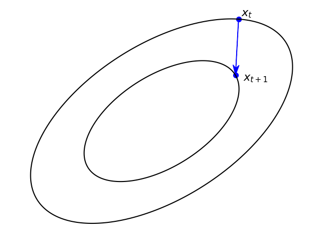
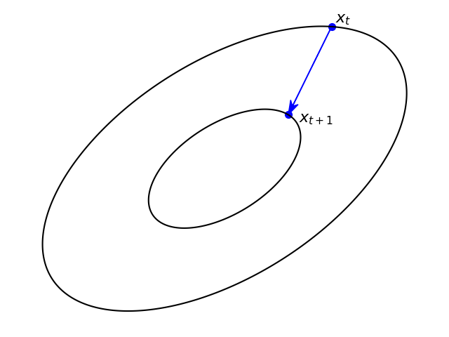
Recalling that the gradient is orthogonal (perpendicular) to its level contour, the following pair of images provides a visual insight into the difference between the two approaches (generated by this code).


Gradient step - perpendicular to the level contour at \(x_t\).	Proximal step - perpendicular to the level contour at \(x_{t+1}\).

The proximal step makes a ‘straight shot’ toward the next, hopefully lower level contour. So, intuitively, it is less probable to miss with a step-size which is a bit too large, and thus is stable w.r.t the step-size choice.

The Moreau envelope viewpoint

Let’s assume, for simplicity, that \(f\) is convex, since the results provide a nice intuition. In the last post, we saw that the proximal point step in equation (PP) above can be alternatively writte using Moreau’s proximal operator:

\[x_{t+1} = \operatorname{prox}_{\eta f}(x_t)\]

We also saw that the gradient of \(M_{\eta} f\), the Moreau envelope of \(f\), is given by the formula

\[\nabla M_\eta f(x) = \frac{1}{\eta}(x - \operatorname{prox}_{\eta f}(x)),\]

which can be re-arranged into

\[\operatorname{prox}_{\eta f}(x) = x - \eta \nabla M_\eta f(x).\]

So, the proximal point method is, in fact:

\[x_{t+1} = x_t - \eta \nabla M_{\eta} f(x_t).\]

Whoa! So, it seems that the proximal point step is nothing but the gradient step, but applied to the Moreau envelope of the loss, instead of the loss itself. In other words, it seems that the stochastic proximal point algorithm is just SGD with each loss replaced by its Moreau envelope. Why should we apply SGD to the envelopes of the incurred losses, instead of the losses themselves? That will become apparent in the next section.

Smoothness, and the role of the proximity component

Both SGD-type methods and the proximal point method share a common structure:

\[x_{t+1} = \operatorname*{argmin}_x \left\{ \color{blue}{\text{approx. of the loss}} + \color{red}{\text{proximity to } x_t} \right\}\]

We know the role of the blue part - its role is to carry information about the loss w.r.t the current training sample. But what is the role of the proximity term? Well, recall that our aim is to optimize the entire average

\[F(x)= \frac{1}{n} \sum_{i=1}^n f_i(x)\]

and not just the loss incurred by one training sample \(f \in \{ f_1,\dots, f_n \}\). How do we know how close we are to minimizing \(F\)? Well, at optimality we certainly should have \(\nabla F(x) = 0\), so one natural measure of ‘how far away from optimality are we’, which we call an optimality gap, is the gradient norm \(\| \nabla F(x) \|\). Another optimality gap may be \(F(x) - \inf_x F(x)\), namely, how far away is the function value at \(x\) from the optimal value?

In contrast to the blue part, the red part’s role is carrying information about the entire average \(F\) by providing a bound on ‘how much would we ruin the optimality gap by moving from \(x_t\) to \(x\)?’. So each iteration in fact is about balancing between decreasing the loss incurred by the current training sample, while avoiding ruining the optimality gap for the entire training set. A properly chosen step-size will create such balance between the two opposing forces such that the iteration sequence will drive \(F\) towards optimality.

Now let’s do some hand-waving, without any formal analysis. Both methods use the weighted squared Euclidean norm \(\frac{1}{2 \eta}\| x - x_t\|_2^2\) as their proximity measure, meaning that they assume that it can somehow bound our optimality gap at \(x\) versus \(x_{t}\). The above is not true in general, but it is true for functions whose gradient changes slowly: if we take two nearby points, the gradients at these points are close to each other well. In formal language, papers occasionally say that \(F\) has a Lipschitz-continuous gradient.

So now let’s get back to the Moreau envelope viewpoint. A remarkable property of Moreau envelopes of convex functions is that they indeed possess the above-mentioned property of having a Lipschitz continuous gradient, and therefore comprise perfect candidates for applying SGD-type methods. Readers who are interested in reading a more formal and rigorous introduction to Moreau envelopes and proximal operators and their relationships to optimization are encouraged to read this or that book, or this excellent tutorial.

Teaser

As promised, we are going to use the fundamentals we have so far to develop proximal-point based algorithms for more advanced scenarios, such as training factorization machines and neural networks, and handle the mini-batch setting. Stay tuned!