“Keeping the polynomial monster under control"
A recap
In the previous post we we saw that the Bernstein polynomials can be used to fit a high-degree polynomial curve with ease, without its shape going out of control. In this post we’ll look at the Bernstein polynomials in more depth, both experimentally and theoretically. First, we will explore the Bernstein polynomials \(\mathbb{B}_n = \{ b_{0,n}, \dots, b_{n, n} \}\), where
\[b_{i,n}(x) = \binom{n}{i} x^i (1-x)^{n-i},\]empirically and visually. We will see how to use the coefficients to achieve a higher degree of control over the shape of the function we fit. Then, we’ll explore them more theoretically, and see that they are indeed a basis - they represent the same model class as the classical power basis \(\{1, x, x^2, \dots, x^n\}\). All the results are reproducible from this notebook.
Shape preserving properties
To study the shape preserving properties, we will rely on the bernvander function we’ve implemented in the last post, that given the numbers \(x_1, \dots, x_m\), computes the Bernstein Vandermonde matrix of a given degree \(n\), that contains all the polynomials evaluated at all the given points:
This is something we should have probably done earler, but let’s plot the Bernstein polynomials to see what they look like. Below, we plot the basis \(\mathbb{B}_{7}\) using the bernvander function.
import matplotlib.pyplot as plt
import numpy as np

plt_xs = np.linspace(0, 1, 1000)
bernstein_basis = bernvander(plt_xs, deg=7)

plt.plot(plt_xs, bernstein_basis,
         label=[f'$b_{{{i},8}}$' for i in range(8)])
plt.legend(ncols=2)
plt.show()
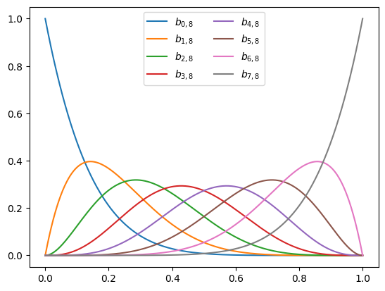
We can see that each polynomial is a “hill” whose maxima appear equally spaced. So are they? Let’s add vertical bars using the axvline function to verify:
plt_xs = np.linspace(0, 1, 1000)
bernstein_basis = bernvander(plt_xs, deg=7)

plt.plot(plt_xs, bernstein_basis,
         label=[f'$b_{{{i},8}}$' for i in range(8)])
for x in np.linspace(0, 1, 8):
  plt.axvline(x, color='gray', linestyle='dotted')
plt.legend(ncols=2)
plt.show()
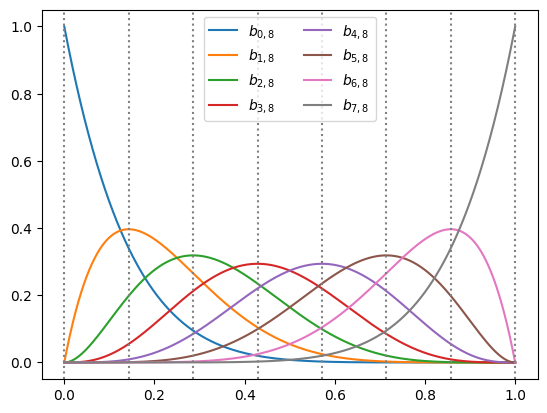
It indeed appears so - the maxima of the polynomials are at \(\{ \tfrac{i}{n}\}_{i=0}^n\). We won’t prove it formally, but that’s not hard. Now we can have some interesting insights. Suppose we have a polynomial written in Bernstein form, namely, as a weighted sum of Bernstein polynomials:
\[f(x) = \sum_{k=0}^n u_i b_{i,n}(x)\]Recall from the previous post that the Bernstein polynomials sum to one, and therefore \(f(x)\) is just a weighted average of the coefficients \(u_0, \dots, u_n\). Thus, at \(x=\frac{i}{n}\), the weight of \(u_i\) in the weighted average dominates the weights of the other coefficients. In other words,
\(u_i\) controls the polynomial \(f(x)\) in the vicinity of the point \(\frac{i}{n}\).
In fact, the name often given to the coefficients \(u_0, \dots, u_n\) is “control points”. To visualize this observation, let’s see what happens if we change one coefficient, \(u_3\), of a 7-th degree polynomial using an animation:
from matplotlib.animation import FuncAnimation, PillowWriter

n = 7
n_frames = 50

ctrl_xs = np.linspace(0, 1, 1 + n)      # the points i / n
w_init = np.cos(2 * np.pi * ctrl_xs)    # initial coefficients
plt_vander = bernvander(plt_xs, deg=n)  # bernstein basis at plot points

fig, ax = plt.subplots()
def animate(i):
  # animate the coefficients "w"
  t = np.sin(2 * np.pi * i / n_frames)
  w = np.array(w_init)
  w[3] = (1 - t) * w[3] + t * 3

  # plot the Bernstein polynomial and the coefficients at i / n
  ax.clear()
  ax.set_xlim([-0.05, 1.05])
  ax.set_ylim([-3, 3])
  control_plot = ax.scatter(ctrl_xs, w, color='red')        # plot control points
  poly_plot = ax.plot(plt_xs, plt_vander @ w, color='blue') # plot the polynomial
  return poly_plot, control_plot

ani = FuncAnimation(fig, animate, n_frames)
ani.save('control_coefficients.gif', dpi=300, writer=PillowWriter(fps=25))
We get the following result:
Looks nice! We can indeed see where the name “control points” comes from. But what can we say about it formally? Well, there are several results. The most famous one is the constructive proof of the Weierstrass approximation theorem:
Theorem [Lorentz1, 1952] Suppose \(g(x)\) is continuous in \([0, 1]\). Then the polynomials \(\sum_{i=0}^n g(\tfrac{i}{n}) b_{i,n}(x)\) uniformly converge to \(g(x)\) as \(n \to \infty\).
As a consequence, we can interpret the Bernstein coefficient \(u_i\) as the value of some function \(g\) that our polynomial approximates at \(x=\frac{i}{n}\). Equipped with this idea, we can ask ourselves a simple question. What if the coefficients are increasing? Will the polynomial be an increasing function?
Well, it turns out the answer is yes - we can force the polynomial to be an increasing function of \(x\) by making sure the coefficients are increasing. In fact, we have even more interesting things we can formally say. To do that, let’s look at the derivatives of polynomials in Bernstein form. Suppose that
\[f(x) = \sum_{i=0}^n u_i b_{i,n}(x),\]then the first and second derivatives are:
\[\begin{align} f'(x) &= n \sum_{i=0}^{n-1} (u_{i+1} - u_i) b_{i,n-1}(x) \\ f''(x) &= n (n-1) \sum_{i=0}^{n-2} (u_{i+2} - 2 u_{i+1} + u_i) b_{i,n-2}(x) \end{align}\]The first derivative is a weighted sum of the coefficient first order differences \(u_{i+1}-u_i\), whereas the second derivative is a weighted sum of the second order differences \(u_{i+2}-2u_{i+1}+u_i\). Therefore, we can conclude that:
Theorem [Chang et. al2, 2007, Proposition 1] Given \(f(x) = \sum_{i=0}^n u_i b_{i,n}(x)\)
- If \(u_{i+1} - u_i \geq 0\), then \(f'(x) \geq 0\), and \(f\) is nondecreasing,
- If \(u_{i+1} - u_i \leq 0\), then \(f'(x) \leq 0\), and \(f\) is nondecreasing,
- If \(u_{i+2} - 2u_{i+1} + u_i \geq 0\), then \(f''(x) \geq 0\), and \(f\) is convex,
- If \(u_{i+2} - 2u_{i+1} + u_i \leq 0\), then \(f''(x) \leq 0\), and \(f\) is concave,
An important application of fitting nondecreasing functions, for example, is fitting a CDF. One practical example of CDF fitting is the bid shading problem345 in online advertising. We are required to model the probability of winning an ad auction given a bid \(x\). Naturally, the winning probability should increase when the bid \(x\) increases. Another important example is calibration curves678 in classification models, which are functions that map the model’s score to a probability such that the mean predicted probability conforms to the true conditional probability of the label given the features. The curve should be increasing - the higher the score, the higher probability it represents. See this great tutorial in the SkLearn documentation.
The simplest way to impose constraints on the coefficients when fitting models on small-scale data is using the CVXPY library, which we already encountered in previous posts in this blog. The library allows solving arbitrary convex optimization problems, specified by the function to minimize, and a set of constraints. Let’s see how we can use CVXPY to fit a nondecreasing Bernstein polynomial. First, we define the function and use it to generate noisy data:
def nondecreasing_func(x):
  return (3 - 2 * x) * (x ** 2) * np.exp(x)

# define number of points and noise
m = 30
sigma = 0.2

np.random.seed(42)
x = np.random.rand(m)
y = nondecreasing_func(x) + sigma * np.random.randn(m)
Now, we define the model fitting as an optimization problem with constraints. Mathematically, we aim to minimize the L2 loss subject to coefficient monotonicity contstraints:
\[\begin{align} \min_{\mathbf{u}} & \quad \| \mathbf{V} \mathbf{u} - \mathbf{y} \|^2 \\ \text{s.t.} &\quad u_{i+1} \geq u_i && i = 0, \dots, n-1 \end{align}\]The matrix \(\mathbf{V}\) is the Bernsten Vandermonde matrix at \(x_1, \dots, x_m\). When multiplied by \(\mathbf{u}\) we obtain the values of the polynomials in Bernstein form at each of the data points. The following CVXPY code is just a direct formulation of the above for fitting a polynomial of degree \(n=20\):
import cvxpy as cp

deg = 20
u = cp.Variable(deg + 1)                          # a placeholder for the optimal Bernstein coefficients
loss = cp.sum_squares(bernvander(x, deg) @ u - y) # The L2 loss - the sum of residual squares
constraints = [cp.diff(u) >= 0]                   # constraints - u_{i+1} - u_i >= 0
problem = cp.Problem(cp.Minimize(loss), constraints)

# solve the minimization problem and
problem.solve()
u_opt = u.value
Now, let’s plot the points, the original, and the fit functions:
plt.scatter(x, y, color='red')
plt.plot(plt_xs, nondecreasing_func(plt_xs), color='blue')
plt.plot(plt_xs, bernvander(plt_xs, deg) @ u_opt, color='green')
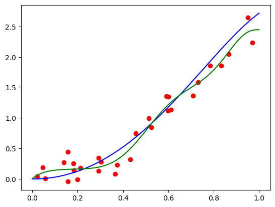
Not bad, given the level of noise, and the fact that we have no regularization whatsoever! For larger scale problems we will typically use an ML framework, such as PyTorch or Tensorflow, and they do not provide mechanisms to impose hard constraints on parameters. Therefore, when using such frameworks, we need to use a regularization term that penalizes violation of our desired constraints. For example, to penalize for violating the nondecreasing constraint, we can use the regularizer:
\[r(\mathbf{u}) = \sum_{i=1}^n \max(0, u_{i} - u_{i+1})^2\]Looking at the curve above, we see that it’s a bit wiggly. Can we do something about it? Looking at the the second derivative formula above, we can “smooth out” the curve by adding a regularization term that penalizes the second order differences. This will, in turn, penalize the second order derivative. Why second order? Because ideally, when the second order differences are zero, we’ll get a straight line. So we’re “smoothing out” the curve to be more straight.
Mathematically, we’ll need to solve:
\[\begin{align} \min_{\mathbf{u}} & \quad \| \mathbf{V} \mathbf{u} - \mathbf{y} \|^2 + \alpha \sum_{i=0}^{n-2} (u_{i+2} - 2 u_{i+1} - u_i)^2 \\ \text{s.t.} &\quad u_{i+1} \geq u_i && i = 0, \dots, n-1 \end{align}\]where \(\alpha\) is a tuned regularization parameter. The code in CVXPY, after tuning \(\alpha\), looks like this:
deg = 20
alpha = 2

u = cp.Variable(deg + 1)                          # a placeholder for the optimal Bernstein coefficients
loss = cp.sum_squares(bernvander(x, deg) @ u - y) # The L2 loss - the sum of residual squares
reg = alpha * cp.sum_squares(cp.diff(u, 2))       # penalty for 2nd order differences
constraints = [cp.diff(u) >= 0]                   # constraints - u_{i+1} - u_i >= 0
problem = cp.Problem(cp.Minimize(loss + reg), constraints)
After solving the problem and plotting the polynomial, I obtained this:

Not bad! Now we will study the Bernstein basis from a more theoretical perspective to understand their representation power.
The Bernstein polynomials as a basis
So, is it really a basis? First, let’s note the set \(\mathbb{B}_n\) of n-th degree Bernstein poynomials indeed has \(n+1\) polynomial functions. So it remains to be convinced that any polynomial can be expressed as a weighted sum of these \(n+1\) functions. It turns out that for any \(k < n\), we can write:
\[x^k = \sum_{j=k}^n \frac{\binom{j}{k}}{\binom{n}{k}} b_{j, n}(x) = \sum_{j=k}^n q_{j,k} b_{j,n}(x)\]The proof is a bit technical and involved, and requires the inverse binomial transform, but it gives us our desired result: any power of \(x\) up to \(n\) can be expressed using Bernstein polynomials. Consequently, any polynomial of degree up to \(n\) can be expressed as a weighted sum of Bernstein polynomials, and therefore:
The representation power of Bernstein polynomials is identical to that of the standard basis. Both represent the same model class we fit to data.
Using Bernstein polynomials, in itself, does not restrict or regularize the model class, since any polynomial can be written in Bernstein form. The Bernstein form is just easier to regularize.
This observation leads to some interesting insights, which will be easier to describe by writing the standard and the the Bernstein bases as vectors:
\[\mathbf{p}_n(x)=(1, x, x^2, \cdots, x^n)^T, \qquad \mathbf{b}_n(x)=(b_{0,n}(x), \cdots, b_{n,n}(x))^T\]We note that the standard and Bernstein Vandermonde matrix rows we saw in the previous post are exactly \(\mathbf{p}_n(x_i)\), and \(\mathbf{b}_n(x_i)\), respectively. Using this notation, we can write the powers of \(x\) in terms of the Bernstein basis in matrix form, by gathering the coefficients \(q_{j,k}\) above, assuming that \(q_{j,k}=0\) whenever \(j<k\), into a triangular matrix \(\mathbf{Q}_n\):
\[\mathbf{p}_n(x)^T = \mathbf{b}_n(x)^T \mathbf{Q}_n\]The matrix \(\mathbf{Q}_n\) is the basis trasition matrix - it can transform any polynomial written using the standard basis to the same polynomial written in the Bernstein basis:
\[a_0 + a_1 x + \dots + a_n x^n = \mathbf{p}_n(x)^T \mathbf{a} = \mathbf{b}_n(x)^T \mathbf{Q}_n \mathbf{a}\]The vector \(\mathbf{Q}_n \mathbf{a}\) is s the coefficient vector w.r.t the Bernstein basis. Does it mean we can actually fit a polynomial in the standard basis, but regularize it as if it was written in the Bernstein basis? Well, yes we can! Polynomial fitting in the Bernstein basis can be written as
\[\min_{\mathbf{w}} \quad \frac{1}{2}\sum_{i=1}^n (\mathbf{b}_n(x_i) \mathbf{w} - y_i)^2 + \frac{\alpha}{2} \| \mathbf{w} \|^2.\]The constants \(\frac{1}{2}\) are for convenience later, when taking derivatives. Introducing the change of variables \(\mathbf{w} = \mathbf{Q}_n \mathbf{a}\), the above problem becomes equivalent to:
\[\min_{\mathbf{a}} \quad \frac{1}{2} \sum_{i=1}^n (\mathbf{p}_n(x_i) \mathbf{a} - y_i)^2 + \frac{\alpha}{2} \| \mathbf{Q}_n \mathbf{a} \|^2. \tag{P}\]Thus, we can fit a polynomial in terms of its standard basis coefficients \(\mathbf{a}\), but regularize its Bernstein coefficients \(\mathbf{Q}_n \mathbf{a}\). So does it really work? Let’s check! First, let’s implement the transition matrix function:
import numpy as np
from scipy.special import binom

def basis_transition(n):
  ks = np.arange(0, 1 + n)
  js = np.arange(0, 1 + n).reshape(-1, 1)
  Q = binom(js, ks) / binom(n, ks)
  Q = np.tril(Q)
  return Q
The regularized least-squares problem (P) above is a convex problem that can be easily solved by equating the gradient w.r.t \(\mathbf{a}\) with zero. Putting all the \(\mathbf{p}_n(x_i)\) for the data points \(i = 1, \dots, m\) into the rows of the Vandermonde matrix \(\mathbf{V}\), equating the gradient to zero becomes:
\[\mathbf{V}^T (\mathbf{V} \mathbf{a} - \mathbf{y}) + \alpha \mathbf{Q}_n^T \mathbf{Q}_n \mathbf{a} = 0.\]Re-arranging, and solving for the coefficients \(\mathbf{a}\), we obtain:
\[\mathbf{a} = (\mathbf{V}^T \mathbf{V} + \alpha \mathbf{Q}_n^T \mathbf{Q}_n)^{-1} \mathbf{V}^T \mathbf{y}\]So let’s implement the fitting procedure:
import numpy.polynomial.polynomial as poly

def fit_bernstein_reg(x, y, alpha, deg):
  """ Fit a polynomial in the standard basis to the data-points `(x[i], y[i])` with Bernstein
      regularization `alpha`, and degree `deg`.
  """
  V = poly.polyvander(x, deg)
  Q = basis_transition(deg)

  A = V.T @ V + alpha * Q.T @ Q
  b = V.T @ y

  # solve the linear system
  a = np.linalg.solve(A, b)
  return a
Now, let’s try reproducing the results of the previous post with degrees 50 and 100.
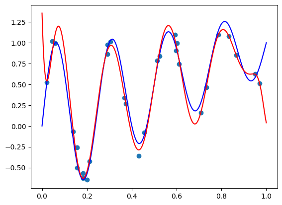
def true_func(x):
  return np.sin(8 * np.pi * x) / np.exp(x) + x

# define number of points and noise
m = 30
sigma = 0.1
deg = 50

# generate features
np.random.seed(42)
x = np.random.rand(m)
y = true_func(X) + sigma * np.random.randn(m)

# fit the polynomial
a = fit_bernstein_reg(x, y, 5e-4, deg=deg)

# plot the original function, the points, and the fit polynomial
plt_xs = np.linspace(0, 1, 1000)
polynomial_ys = poly.polyvander(plt_xs, deg) @ a
plt.scatter(x, y)
plt.plot(plt_xs, true_func(plt_xs), 'blue')
plt.plot(plt_xs, polynomial_ys, 'red')
plt.show()
I got the following plot, which appears pretty similar to what we got in the previous post, but slightly worse:

Let’s crank up the degree to 100 by setting deg = 100. I got the following image:
Again, slightly worse than what we achieved by directly fitting the Bernstein form, but appears close.
There two technical issues with our idea. First, manually fitting models rather than relying on standard tools, such as SciKit-Learn appears to be troublesome, and in terms of computational efficiency, we need to deal with the additional matrix \(\mathbf{Q}_n\). Second, and most importantly, the standard Vandermonde matrix and the basis transition matrix \(\mathbf{Q}_n\) are extremely ill conditioned. This makes hard to actually solve the fitting problem and obtain coefficients that are close to the true optimal coefficients. This is true regardless if we chose direct matrix inversion, CVXPY, or an SGD-based optimizer from PyTorch or TensorFlow.
Due to inefficiency and ill conditioning this trick has a little value in practice. But provides us with an important insight: achieving good regularization requires a sophisticated non-diagonal matrix in the regularization term. It’s not a formal statement, but probably any “good” basis will have a non-diagonal transition matrix to the standard basis. This means that fitting a polynomial in the standard basis using typical ML tricks of rescaling the columns of the Vandermonde matrix has a little chance of success. And it doesn’t matter if we rescale using min-max scaling, or standardization to zero mean and unit variance. To fit a polynomial, we need to use a “good” basis directly.
Conclusion
In this post we explored the ability of the Bernstein form to control the shape of the curve we’re fitting - either making it smooth, increasing, decreasing, convex, or concave. Then, we saw that Bernstein polynomials are just polynomials - they have the same representation power as the standard basis, but just easier to regularize.
The next post will be more engineering oriented. We’ll see how to use the Bernstein basis for feature engineering and fitting models to some real-world data-sets, and we will write a SciKit-Learn transformer to do so. Stay tuned!
-
Lorentz, G. G. (1952). Bernstein Polynomials. University of Toronto Press. ↩
-
Chang, I. S., Chien, L. C., Hsiung, C. A., Wen, C. C., & Wu, Y. J. (2007). Shape restricted regression with random Bernstein polynomials. Lecture Notes-Monograph Series, 187-202. ↩
-
Sarah Sluis, S. (2019). Everything you need to know about bid shading. ↩
-
Karlsson, N., & Sang, Q. (2021, May). Adaptive bid shading optimization of first-price ad inventory. In 2021 American Control Conference (ACC) (pp. 4983-4990). IEEE. ↩
-
Gligorijevic, D., Zhou, T., Shetty, B., Kitts, B., Pan, S., Pan, J., & Flores, A. (2020, October). Bid shading in the brave new world of first-price auctions. In Proceedings of the 29th ACM International Conference on Information & Knowledge Management (pp. 2453-2460). ↩
-
Niculescu-Mizil, A., & Caruana, R. (2005, August). Predicting good probabilities with supervised learning. In Proceedings of the 22nd international conference on Machine learning (pp. 625-632). ↩
-
Platt, J. (1999). Probabilistic outputs for support vector machines and comparisons to regularized likelihood methods. Advances in large margin classifiers, 10(3), 61-74. ↩
-
Zadrozny, B., & Elkan, C. (2002, July). Transforming classifier scores into accurate multiclass probability estimates. In Proceedings of the eighth ACM SIGKDD international conference on Knowledge discovery and data mining (pp. 694-699). ↩