“SkLearning with Bernstein Polynomials"
This post is part of the series "Polynomial features in machine learning", and is not self-contained.
Series posts:
-
“Are polynomial features the root of all evil?"
-
“Keeping the polynomial monster under control"
- “SkLearning with Bernstein Polynomials" (this post)
-
SkLearning with Bernstein Polynomials - continued
-
A Bernstein SkLearn model calibrator
-
Regularization properties of polynomial bases
-
Let the polynomial monster free
-
Off with the polynomial's tail!
-
Paying attention to feature distribution alignment
- “Are polynomial features the root of all evil?"
- “Keeping the polynomial monster under control"
- “SkLearning with Bernstein Polynomials" (this post)
- SkLearning with Bernstein Polynomials - continued
- A Bernstein SkLearn model calibrator
- Regularization properties of polynomial bases
- Let the polynomial monster free
- Off with the polynomial's tail!
- Paying attention to feature distribution alignment
Intro
In the last two posts we introducted the Bernstein basis as an alternative way to generate polynomial features from data. In this post we’ll be concerned with an implementation that we can use in our model training pipelines based on Scikit-Learn. The Scikit-Learn library has the concept of a a transformer class that generates features from raw data, and we will indeed develop and test such a transformer class for the Bernstein basis. Contrary to previous posts, here we will have some math, but plenty of code, which is fully available in this Colab Notebook.
But beforehand, let’s do a short recap of what we learned in the last two posts:
- The Bernstein basis is a useful alternative to the standard polynomial basis \(\{1, x, x^2, \dots, x^n\}\). It has a well conditioned Vandermonde matrix, and is easy to regularize.
- Any polynomial basis has a “natural domain” where its approximation properties are well-known. Raw features must be normalized to that domain. The natural domain of the Bernstein basis is the interval \([0, 1]\).
- Extrapolation outside the training data distribution is not a problem - we can impose smoothness via regularization.
- Extrapolation outside the “natural domain” should be avoided!1
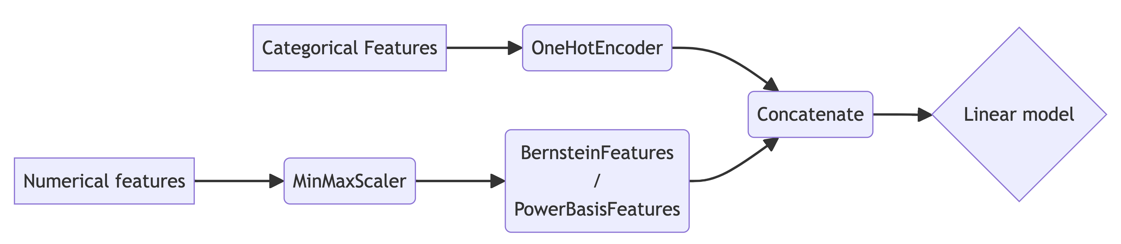
Transformer classes in Scikit-Learn generate new features out of existing ones, and can be combined in a convenient way into pipelines that perform a set of transformations that eventually generate features for a trained model. We will implement a Scikit-Learn transformer class for Bernstein polynomials, called BernsteinFeatures. As a baseline, we will also implement a similar transformer that generates the power basis, called PowerBasisFeatures. We will combine them in a Pipeline to build a mechainsm that trains and evaluates a model using the well-known fit-transform paradigm. In this post, we will train a linear model on our generated features.
Since feature normalization is a must, we will always prepend our polynomial transformer by a normalization transformer. In this post, we will use the MinMaxScaler class built into Scikit-Learn. For categorical features, we will use OneHotEncoder. Therefore, our pipelines in this post will have the following generic form:
Before we begin - some expectations. The behavior of the functions we approximate on real data-sets is typically not as ‘crazy’ as the toy functions we approximated in previous posts. The wide oscilations and wiggling of the “true” function we are aiming to learn are not that common in practice. A harder challenge is modeling the interaction between several features, rather than the effect of each feature separately. Therefore, the advantage we will see from a simple application of Bernstein polynomials over the power basis isn’t that large, but it’s quite visible and consistent. Thus, when fitting a model with polynomial features, I’d go with Bernstein polynomials by default, instead of a power basis. It’s very easy, and we have nothing to lose - we can only gain.
The transformer classes
A transformer class in Scikit-Learn needs to implement the basic fit-transform paradigm. Since polynomial features are the same regardless of the data, the fit method is empty. The transform method, as expected, will concatenate the generate a Vandermonde matrices of the columns. Note, that we will be handling each column separately at this stage, and do not aim to compute any interaction terms between columns.
There is one mathematical issue we need to take care of. Since a polynomial basis can represent any polynomial, including those that do not pass throught the origin, they implicitly contain a “bias” term. The power basis even explicit about it - its first basis function is the constant \(1\). However, a typical linear model already has its own bias term, namely,
\[f(\mathbf{x}) = \langle \mathbf{w}, \mathbf{x}\rangle + b.\]The bias is, of course, equivalent to having a constant feature. Thus, our data-matrix has two constant features, meaning it’s as ill-conditioned as it can be - its columns are linearly dependent. When several numerical features are used things become even worse - we have several implicit constant features.
To mitigate the above, we will add a bias boolean flag to our transformers that instructs the transformer to generate a basis of polynomials going through the origin. This policy is in line with other transformers that are built-in into Scikit-Learn, such as the SplineTransformer and the PolynomialFeatures classes. For the power basis it amounts to discarding the first basis function. It turns out that the same idea works for the Bernstein basis as well, since \(b_{0,n}(0) = 1\), and \(b_{i,n}(0) = 0\) for all \(i \geq 1\).
Becide the above mathematical aspect, we will also have to take care of several technical aspects. First, we will add support for Pandas data-frames, since they are ubiquitously used by many practitioners. Second, we will have to take care of one-dimensional arrays as input, and reshape them into a column. Finally, we will treat transform NaN values to constant (zero) vectors to model the fact that a missing numerical feature “has no effect”. This is not always the best course of action, but it’s useful in this post. The base class taking care of the above mathematical and technical aspects is written below:
import numpy as np
from sklearn.base import BaseEstimator, TransformerMixin


class PolynomialBasisTransformer(BaseEstimator, TransformerMixin):
    def __init__(self, degree=5, bias=False, na_value=0.):
        self.degree = degree
        self.bias = bias
        self.na_value = na_value

    def fit(self, X, y=None):
        return self

    def transform(self, X, y=None):
        # Check if X is a Pandas DataFrame and convert to NumPy array
        if hasattr(X, 'values'):
            X = X.values

        # Ensure X is a 2D array
        if X.ndim == 1:
            X = X.reshape(-1, 1)

        # Get the number of columns in the input array
        n_rows, n_features = X.shape

        # Compute the specific polynomial basis for each column
        basis_features = [
            self.feature_matrix(X[:, i])
            for i in range(n_features)
        ]

        # no bias --> skip the first basis function
        if not self.bias:
            basis_features = [basis[:, 1:] for basis in basis_features]

        return np.hstack(transformed_features)

    def feature_matrix(self, column):
      vander = self.vandermonde_matrix(column)
      return np.nan_to_num(vander, self.na_value)

    def vandermonde_matrix(self, column):
        raise NotImplementedError("Subclasses must implement this method.")
The power and Bernstein bases are easily implemented by overriding the vandermonde_matrix method of the above base-class:
import numpy.polynomial.polynomial as poly
from scipy.stats import binom

class BernsteinFeatures(PolynomialBasisTransformer):
    def vandermonde_matrix(self, column):
        basis_idx = np.arange(1 + self.degree)
        basis = binom.pmf(basis_idx, self.degree, column[:, None])
        return basis


class PowerBasisFeatures(PolynomialBasisTransformer):
    def vandermonde_matrix(self, column):
        return poly.polyvander(column, self.degree)
Let’s see how they work. We will use Pandas to display the results of our transformers as nicely formatted tables.
import pandas as pd

pbt = BernsteinFeatures(degree=2).fit(np.empty(0))
bbt = PowerBasisFeatures(degree=2).fit(np.empty(0))

# transform a column - output the Vandermonde matrix according to each basis
feature = np.array([0, 0.5, 1, np.nan])
print(pd.DataFrame.from_dict({
    'Feature': feature,
    'Power basis': list(pbt.transform(feature)),
    'Bernstein basis': list(bbt.transform(feature))
}))

# transform a column - output the Vandermonde matrix according to each basis
feature = np.array([0, 0.5, 1, np.nan])
print(pd.DataFrame.from_dict({
    'Feature': feature,
    'Power basis': list(pbt.transform(feature)),
    'Bernstein basis': list(bbt.transform(feature))
}))
#    Feature                 Power basis Bernstein basis
# 0      0.0                  [0.0, 0.0]      [0.0, 0.0]
# 1      0.5  [0.5000000000000002, 0.25]     [0.5, 0.25]
# 2      1.0                  [0.0, 1.0]      [1.0, 1.0]
# 3      NaN                  [0.0, 0.0]      [0.0, 0.0]

# transform two columns - concatenate the Vandermonde matrices
features = np.array([
    [0, 0.25],
    [0.5, 0.5],
    [np.nan, 0.75]
])
print(pd.DataFrame.from_dict({
    'Feature 0': features[:, 0],
    'Feature 1': features[:, 1],
    'Power basis': list(pbt.transform(features)),
    'Bernstein basis': list(bbt.transform(features))
}))
#    Feature 0  Feature 1                                           Power basis           Bernstein basis
# 0        0.0       0.25                             [0.0, 0.0, 0.375, 0.0625]  [0.0, 0.0, 0.25, 0.0625]
# 1        0.5       0.50  [0.5000000000000002, 0.25, 0.5000000000000002, 0.25]    [0.5, 0.25, 0.5, 0.25]
# 2        NaN       0.75                             [0.0, 0.0, 0.375, 0.5625]  [0.0, 0.0, 0.75, 0.5625]
Nice! Now let’s proceed to our example.
Model training components
Let’s implement the pipeline structure we saw at the beginning of this post in code, and a function to train models using this pipeline.
Training pipeline
We will write a function that a basis transformer and a model as an arguments, and constructs the components of the pipeline. Categorical features will be one-hot encoded, numerical features will be scaled and transformed using the given basis transformer, and finally the result will be passed as an input of the given model.
To make sure our scaled numerical features never fall outside of the \([0, 1]\) interval, even if the test-set contaisn values larger or smaller than what we saw in the training set, we clip the scaled value to \([0, 1]\). And to make sure we don’t inflate the dimension of our model by one-hot encoding rare categorical values, we will limit their frequency to 10. Here is the code:
from sklearn.pipeline import Pipeline
from sklearn.preprocessing import OneHotEncoder, MinMaxScaler
from sklearn.compose import ColumnTransformer

def training_pipeline(basis_transformer, model_estimator,
                      categorical_features, numerical_features):
  basis_feature_transformer = Pipeline([
      ('scaler', MinMaxScaler(clip=True)),
      ('basis', basis_transformer)
  ])

  categorical_transformer = OneHotEncoder(
      sparse_output=False,
      handle_unknown='infrequent_if_exist',
      min_frequency=10
  )

  preprocessor = ColumnTransformer(
      transformers=[
        ('numerical', basis_feature_transformer, numerical_features),
        ('categorical', categorical_transformer, categorical_features)
      ]
  )

  return Pipeline([
    ('preprocessor', preprocessor),
    ('model', model_estimator)
  ])
We can now use a pipeline with Bernstein features with Ridge regression as in:
pipeline = training_pipeline(BernsteinFeatures(), Ridge(), categorical_features, numerical_features)
test_predictions = pipeline.fit(train_df, train_df[target]).transform(test_df)
But wait! We need to know what polynomial degree to use, and maybe tune some hyperparameters of the trained model. Otherwise, the experimental results we observe may simply be due to a bad choice of hyperparameters.
Tuning hyperparameters
We need two ingredients. One is technical - how we set hyperparameters of components hidden deep inside a Pipeline. The other is how we actually tune them. For setting hyperparameters, Scikit-Learn provides an interface. There are two functions: get_params() which returns a dictionary of all settable parameters, and set_params that can set parameters of all the components contained inside a pipeline. Let’s look at an example of a pipeline with BernsteinFeatures as the basis transformer, and Ridge as the model. Since Ridge has an alpha parameter, and BernsteinFeatures has a degree parameters, let’s look for those:
from sklearn.linear_model import Ridge

pipeline = training_pipeline(BernsteinFeatures(), Ridge(), [], [])
print({k:v for k,v in pipeline.get_params().items()
           if 'degree' in k or 'alpha' in k})
# prints: {'preprocessor__numerical__basis__degree': 5, 'model__alpha': 1.0}
There is a pattern here! Looking at our training_pipeline method above, we see that there is a component named “preprocessor”, inside of which there is a component named “numerical”, that contains a “basis”. That “basis” component is our transformer, so it has a “degree”. The full name is just a concatenation of the above with double underscores. The same idea for the model. We can also set these parameters as follows:
pipeline.set_param('preprocessor__numerical__basis__degree', SOME_DEGREE)
pipeline.set_param('model__alpha', SOME_REGULARIZATION_COEFFICIENT)
So now that we know how to set hyperparameters of parts within a pipeline, let’s tune them. To that end, we will use hyperopt2! It’s a nice hyperparameter tuner, very easy to use, and implementes the state-of-the art Bayesian Optimization paradigm that can obtain high quality hyperparameter configurations hyperparameters in a relatively small number of trials. It’s as easy to use as a grid search, available by default on Colab, and saves us precious time. And I certainly don’t want to wait long until I see the results.
To use hyperopt, we need two ingredients. A a tuning objective that evaluates the performance of a given hyperparameter configuration, and a search space for hyperparameters. Writing such a tuning objective is quite easy - we will use a cross-validated score using Scikit-Learn’s built-int capabilities:
from sklearn.model_selection import cross_val_score

def tuning_objective(pipeline, metric, train_df, target, params):
    pipeline.set_params(**params)
    scores = cross_val_score(pipeline, train_df, train_df[target], scoring=metric)
    return -np.mean(scores)
Well, that wasn’t hard, but there’s an intricate detail - note that we are returning minus the average metric across folds. This is because Scikit-Learn’s metrics are built to be maximized, but hyperopt is built to minimize.
Defining a the hyperparameter seach space is also easy - it’s just a dict specifying a distribution for each hyperparameter. For our example above with a Ridge model we can use something like this:
from hyperopt import hp

param_space = {
    'preprocessor__numerical__basis__degree': hp.uniformint('degree', 1, 50),
    'model__alpha': hp.loguniform('alpha', -10, 5)
}
Hyperopt has a uniform and uniformint functions for hyperparameters that we would normally tune using a uniform grid, such as the number of layers of an NN, or the degree of a polynomial. In the code above, the degree of the polynomial is a number between 1 and 50, and all are equally likely. It also has a loguniform function for hyperparameters that we normally tune using a geometrically-spaced grid, such as a learning rate, or a regularization coefficient. In the example above, the regularization coefficient is between \(e^{-10}\) and \(e^5\), and all exponents are uniformly likely.
Having specified the objective function and the parameter space, we can use fmin for tuning, like this:
from hyperopt import fmin, tpe

fmin(lambda params: tuning_objective(pipeline, metric, train_df, target, params),
     space=param_space,
     algo=tpe.suggest,
     max_evals=100)
We have given it a function to minimize, gave it the hyperparameter search space, told it to use the TPE algorithm for tuning3, and limited it to 100 evaluations of our tuning objective. It will invoke our objective on hyperparameter configurations that it considers as worth trying, and eventually give us the best configuration it found. More on that can be found in hyperopt’s documentation. Beyond the objective and the search space, we also need to tell it which algorithm to use, and how many configurations it should try.
So let’s write a function that tunes hyperparameters using the training set, fits a model using the optimal configuration, and evaluates the resulting model’s performance using the test set. Then, re-train the pipeline on the entire training set using the best hyper-parameters, and evalluate it on the test set.
from hyperopt import fmin, tpe
from sklearn.metrics import get_scorer

def tune_and_evaluate_pipeline(pipeline, param_space,
                               train_df, test_df, target, metric,
                               max_evals=50, random_seed=42):
  print('Tuning params')
  def bound_tuning_objective(params):
    return tuning_objective(pipeline, metric, train_df, target, params)

  params = fmin(fn=bound_tuning_objective, # <-- this is the objective
                space=param_space,         # <-- the search space
                algo=tpe.suggest,          # <-- the algorithm to use. TPE is the most widely used.
                max_evals=max_evals,       # <-- maximum number of configurations to try
                rstate=np.random.default_rng(random_seed),
                return_argmin=False)
  print(f'Best params = {params}')

  print('Refitting with best params on the entire training set')
  pipeline.set_params(**params)
  fit_result = pipeline.fit(train_df, train_df[target])

  scorer = get_scorer(metric)
  score = scorer(fit_result, test_df, test_df[target])
  print(f'Test metric = {score:.5f}')

  return fit_result
Now we have all the ingredients in place! We can now, for example, tune, train a tuned Ridge regression model with Bernstein polynomial features that predicts the foo column in our data-set, and measures success using the Mean-Squared Error metric as follows:
train_df = ...
test_df = ...
categorical_features = [...]
numerical_features = [...]

pipeline = trainin_pipeline(BernsteinTransformer(), Ridge(), categorical_features, numerical_features)
model = tune_and_evaluate_pipeline(
  pipeline,
  param_space,
  train_df,
  test_df,
  'foo',
  'neg_root_mean_squared_error')
Now let’s put our work-horse to work!
California housing price prediction
The well-known California Housing price prediction data-set is available in the samples directory on Colab, so it will be convenient to use. Let’s load it, and print a sample:
train_df = pd.read_csv('sample_data/california_housing_train.csv')
test_df = pd.read_csv('sample_data/california_housing_test.csv')
print(train_df.head())

#    longitude  latitude  housing_median_age  total_rooms  total_bedrooms  population  households  median_income  median_house_value
# 0    -114.31     34.19                15.0       5612.0          1283.0      1015.0       472.0         1.4936             66900.0
# 1    -114.47     34.40                19.0       7650.0          1901.0      1129.0       463.0         1.8200             80100.0
# 2    -114.56     33.69                17.0        720.0           174.0       333.0       117.0         1.6509             85700.0
# 3    -114.57     33.64                14.0       1501.0           337.0       515.0       226.0         3.1917             73400.0
# 4    -114.57     33.57                20.0       1454.0           326.0       624.0       262.0         1.9250             65500.0
The task is predicting the median_house_value column based on the other columns.
First, we can see that there are seveal feature columns with very large and diverse numbers. They probably have a very skewed distribution. Let’s plot those distributions:
skewed_columns = ['total_rooms', 'total_bedrooms', 'population', 'households']
axs = train_df.loc[:, skewed_columns].plot.hist(
    bins=20, subplots=True, layout=(2, 2), figsize=(8, 6))
axs.flat[0].get_figure().tight_layout()
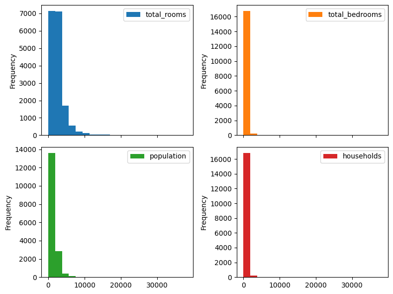
Indeed very skewed! Typically applying a logarithm helps. Let’s see plot them after applying a logarithm (note the .apply(np.log)):
axs = train_df.loc[:, skewed_columns].apply(np.log).plot.hist(
    bins=20, subplots=True, layout=(2, 2), figsize=(8, 6))
axs.flat[0].get_figure().tight_layout()
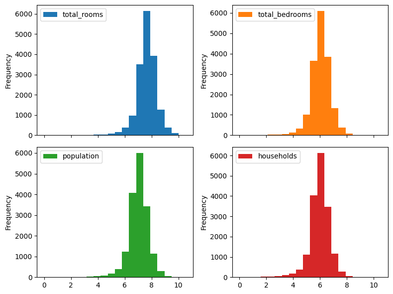
Ah, much better! We also note that housing_median_age variable, despite being numerical, is discrete. Indeed, it has only 52 unitue values in the entire dataset. So we will treat it as a categorical variable. Let’s summarize our features in code:
categorical_features = ['housing_median_age']
numerical_features = ['longitude', 'latitude', 'total_rooms', 'total_bedrooms', 'population', 'households', 'median_income']
target = ['median_house_value']
So we’re almost ready to fit a model. We can see that our target variable, median_house_value , has very large magnitude values. It is usually beneficial to scale them to a smaller range. However, we would like to measure the prediction error with respect to the original values. Fortunately, Scikit-Learn provides us with a TransformedTargetRegressor class that allows scaling the target variable for the regression model, and scaling it back to the original range when producing an output.
Now we’re ready to construct our model fitting pipeline that fits a Ridge model on scaled regression targets, and transformed features:
from sklearn.linear_model import Ridge
from sklearn.compose import TransformedTargetRegressor

def california_housing_pipeline(basis_transformer):
    return training_pipeline(
        basis_transformer,
        TransformedTargetRegressor(
            regressor=Ridge(),
            transformer=MinMaxScaler()
        ),
        categorical_features,
        numerical_features
    )
Beautiful! Now we can use our hyperparameter tuning function to train a tuned model on our dataset. Since it’s a regression task, we will measure the Root Mean Squared Error (RMSE), implemented by the neg_root_mean_squared_error Scikit-Learn metric. So let’s begin with Bernstein polynomial features:
poly_param_space = {
    'preprocessor__numerical__basis__degree': hp.uniformint('degree', 1, 50),
    'model__regressor__alpha': hp.loguniform('C', -10, 5)
}

bernstein_pipeline = california_housing_pipeline(BernsteinFeatures())
bernstein_fit_result = tune_and_evaluate_pipeline(
    bernstein_pipeline, poly_param_space,
    train_df, test_df, target,
    'neg_root_mean_squared_error')
After a few minutes I got the following output:
Tuning params
100%|██████████| 50/50 [03:37<00:00,  4.34s/trial, best loss: 60364.25845777496]
Best params = {'model__regressor__alpha': 0.0075549014272857686, 'preprocessor__numerical__basis__degree': 50}
Refitting with best params on the entire training set
Test metric = -61559.04848
The root mean squared error (RMSE) on the test-set of the tuned model is \(61559.04848\). Now let’s try the power basis:
power_basis_pipeline = california_housing_pipeline(PowerBasisFeatures())
power_basis_fit_result = tune_and_evaluate_pipeline(
    power_basis_pipeline, poly_param_space,
    train_df, test_df, target,
    metric='neg_root_mean_squared_error')
This time I got the following output:
Tuning params
100%|██████████| 50/50 [00:54<00:00,  1.10s/trial, best loss: 62205.78033504614]
Best params = {'model__regressor__alpha': 4.7685837926305776e-05, 'preprocessor__numerical__basis__degree': 31}
Refitting with best params on the entire training set
Test metric = -63534.49228
This time the RMSE is \(63534.49228\). The Bernstein basis got us a \(3.1\%\) improvement! If we look closer at the output, we can see that the tuned Bernstein polynomial is of degree 50, whereas the best tuned power basis polynomial is of degree 31. We already saw that high degree polynomials in the Bernstein basis are easy to regularize, and our tuner probably saw the same phenomenon, and cranked up the degree to 50.
How are our polynomial features compared to a simple linear model? Well, let’s see. To re-use all our existing code instead of writing a new pipeline, we’ll just use a “do nothing” feature transformer that implements the identity function. Note, that this time there is no degree to tune.
class IdentityTransformer(BaseEstimator, TransformerMixin):
    def __init__(self, na_value=0.):
      self.na_value = na_value

    def fit(self, input_array, y=None):
        return self

    def transform(self, input_array, y=None):
        # we are compatible with our polynomial features - NA values are zeroed-out. The rest
        # are passed through
        return np.where(np.isnan(input_array), self.na_value, input_array)

linear_param_space = {
    'model__regressor__alpha': hp.loguniform('C', -10, 5)
}

linear_pipeline = california_housing_pipeline(IdentityTransformer())
linear_fit_result = tune_and_evaluate_pipeline(
    linear_pipeline, linear_param_space,
    train_df, test_df, target,
    'neg_root_mean_squared_error')
Here is the output:
Tuning params
100%|██████████| 50/50 [00:22<00:00,  2.22trial/s, best loss: 66571.41310284132]
Best params = {'model__regressor__alpha': 0.013724898474056764}
Refitting with best params on the entire training set
Test metric = -67627.17474
The RMSE is \(67627.17474\). So let’s summarize the results in the table:
| Linear | Power basis | Bernstein basis | |
|---|---|---|---|
| RMSE | 67627.17474 | 63534.49228 | 61559.04848 |
| Improvement over Linear | 0% | 6.05% | 8.97% |
| Tuned degree | 1 | 31 | 50 |
Impressive! Just changing the polynomial basis gives us a visible boost, and the high degree doesn’t appear to do something bad.
Now we shall inspect our models a bit closer. That’s why we stored the fit models in the bernstein_fit_result and power_basis_fit_result variables above. Following the structure of our pipelines, to get the coefficients we can use the following function:
def get_coefs(pipeline):
  transformed_target_regressor = pipeline.named_steps['model']
  ridge_model = transformed_target_regressor.regressor
  return ridge_model.coef_.ravel()
Now we can plot the polynomials! First, we will need to extract the coefficients of the numerical features, and ignore the ones corresponding to the categorical features. Next, we need to treat the coefficients of each numerical feature separately, and plot the polynomial they represent. Since our numerical features are always scaled to \([0, 1]\), plotting amounts to evaluating our polynomials on a dense grid in \([0, 1]\). So this is our plotting function:
import matplotlib.pyplot as plt

def plot_feature_curves(pipeline, basis_transformer_ctor, numerical_features):
  # get the coefficients and the degree
  degree = pipeline.get_params()['preprocessor__numerical__basis__degree']
  coefs = get_coefs(pipeline)

  # extract the numerical features, and form a matrix, such that the
  # coefficients of each feature is in a separate row.
  numerical_slice = pipeline.get_params()['preprocessor'].output_indices_['numerical']
  feature_coefs = coefs[numerical_slice].reshape(-1, degree)

  # form the basis Vandermonde matrix on [0, 1]
  xs = np.linspace(0, 1, 1000)
  xs_vander = basis_transformer_ctor(degree=degree).fit_transform(xs)

  # do the plotting
  n_cols = 3
  n_rows = math.ceil(len(numerical_features) / n_cols)
  fig, axs = plt.subplots(n_rows, n_cols, figsize=(3 * n_cols, 3 * n_rows))
  for i, (ax, coefs) in enumerate(zip(axs.ravel(), feature_coefs)):
    ax.plot(xs, xs_vander @ coefs)
    ax.set_title(numerical_features[i])
  fig.show()
A bit lengthy, but understandable.
Recalling our previous post, we know that the coefficients in the Bernstein basis are actually “control points”, so let’s add the ability to plot them as well to the above function:
import matplotlib.pyplot as plt

def plot_feature_curves(pipeline, basis_transformer_ctor, numerical_features,
                        plot_control_pts=True):
  # get the coefficients and the degree
  degree = pipeline.get_params()['preprocessor__numerical__basis__degree']
  coefs = get_coefs(pipeline)

  # extract the numerical features, and form a matrix, such that the
  # coefficients of each feature is in a separate row.
  numerical_slice = pipeline.get_params()['preprocessor'].output_indices_['numerical']
  feature_coefs = coefs[numerical_slice].reshape(-1, degree)

  # form the basis Vandermonde matrix on [0, 1]
  xs = np.linspace(0, 1, 1000)
  xs_vander = basis_transformer_ctor(degree=degree).fit_transform(xs)

  # do the plotting
  n_cols = 3
  n_rows = math.ceil(len(numerical_features) / n_cols)
  fig, axs = plt.subplots(n_rows, n_cols, figsize=(3 * n_cols, 3 * n_rows))
  for i, (ax, coefs) in enumerate(zip(axs.ravel(), feature_coefs)):
    if plot_control_pts:
      control_xs = (1 + np.arange(len(coefs))) / len(coefs)
      ax.scatter(control_xs, coefs, s=30, facecolors='none', edgecolor='b', alpha=0.5)
    ax.plot(xs, xs_vander @ coefs)
    ax.set_title(numerical_features[i])
  fig.show()
Now let’s see our Bernstein polynomials!
plot_feature_curves(bernstein_fit_result, BernsteinFeatures, numerical_features)
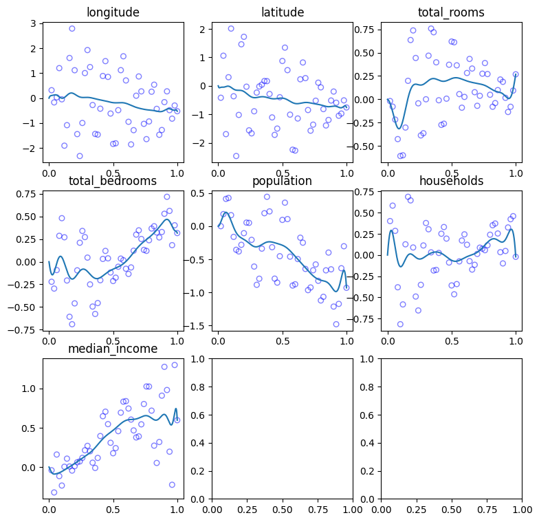
What about the power basis? Let’s take a look as well. Note, that we won’t plot the coefficients as “control points”, since the coefficients of the power basis are not control points in any way.
plot_feature_curves(power_basis_fit_result, PowerBasisFeatures, numerical_features, plot_control_pts=False)
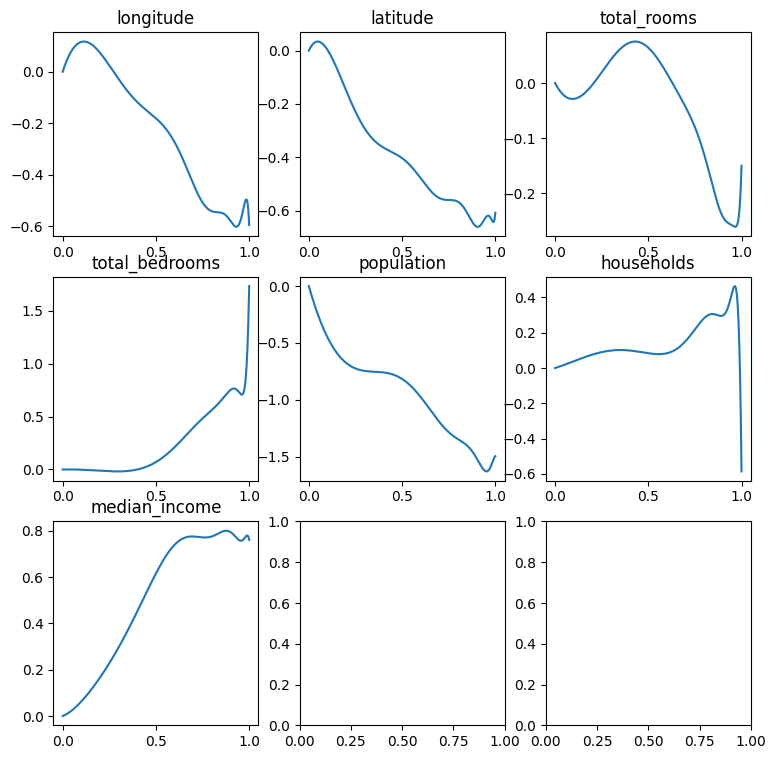
Look at the “households” and “total_bedrooms” polynomials. Seems that they’re “going crazy” near the boundary of the domain. As we expected - was not specifically designed to approximate functions on \([0, 1]\), and it’s hard to regularize to produce a good fit. It will either under-fit, or over-regularize.
In fact, we may recall that the “natural domain” of the power basis is the complex unit circle. It may be interesting to try representing periodic features, such as the time of day using the power basis, since such features naturally map to a point on a circle. However, there are other challenges involved, such as ensuring that our model will be real-valued rather than complex-valued, and this may be a nice subject for another post.
Summary
This was a nice adventure. I certainly learned a lot about Scikit-Learn while writing this post, and I hope that the transformer for producing the Bernstein basis may be useful for to you as well. We note that polynomial non-linear features have a nice property they have only one tunable hyperparameter, so learning a tuned model should be computationally cheaper compared to other alternatives, such as radial basis functions.
Looking again at the Bernstein polynomials above, we see that they are a bit ‘wiggly’, the control point seem like a mess, and in the previous post we learned how to smooth them out by regularizing their second derivative. Moreover, in the beginning of this post we said something interesting - the predictive power of simple models may be improved by incorporating interactions between features. So in the next posts we’re going to do exactly that - enhance our transformer to model feature interactions, and write an enhance version of the Ridge estimator to smooth polynomial features. Stay tuned!
-
I wouldn’t even call it extrapolation - in our context I think of the polynomial basis as “undefined” outside of its natural domain. ↩
-
Bergstra, James, Daniel Yamins, and David Cox. “Making a science of model search: Hyperparameter optimization in hundreds of dimensions for vision architectures.” International conference on machine learning. PMLR, 2013. ↩
-
Watanabe, S., 2023. Tree-structured Parzen estimator: Understanding its algorithm components and their roles for better empirical performance. arXiv preprint arXiv:2304.11127. ↩