Untilting the tilted loss
Intro
Typically in machine learning we train a model by minimizing the average loss over the training set \(\mathbf{x}_1, \dots, \mathbf{x}_n\)1, perhaps with some regularization. Mathematically, we solve the problem:
\[\min_\mathbf{w} \quad \frac{1}{n} \sum_{i=1}^n f(\mathbf{w}, \mathbf{x}_i)\]A recently published JMLR paper2 proposes an alternative, a tilted loss:
\[\min_\mathbf{w} \quad \frac{1}{t} \ln\left( \frac{1}{n} \sum_{i=1}^n \exp(t f(\mathbf{w}, \mathbf{x}_i)) \right)\]The LogSumExp function \(\mathbf{x} \to \ln(\sum_{i=1}^n x_i)\) serves as the “aggregator” of losses over individual samples, instead of just the plain average. The parameter \(t\) can be thought as a kind of ‘temperature’ of our aggregator. When \(t \to \infty\), it converges to the worst-case loss over the training set. This is useful when we want to make sure that we perform reasonably well on the difficult instances as well, and not only on average. Conversely, when \(t \to -\infty\), it converges to the best-case loss over the training set. This is useful for the opposite - perform well on most easy instances, and be less sensitive to “outliers”, or more difficult instances. Taking \(t \to 0\), it converges to the regular average loss. Thus, it allows interpolating between fairness and robustness. For the same of simplicity, in this post we shall assume that \(t > 0\).
Off-the-shelf methods available in PyTorch and TensorFlow are based on stochastic gradients, and are designed to minimize averages over individual samples. However, the tilted loss is not an average due to the LogSumExp aggregation, and hence model training becomes a bit tricky. The paper proposes to use ‘tilted averaging’ on mini-batches, instead of regular averaging, but without a mathematical justification to the best of my knowledge. Intuitively, such strategy minimizes some approximation of the tilted loss, but not the tilted loss itself.
In theory, since a logarithm is monotonic, and \(\frac{1}{t}\) is positive, we could discard both and train on the tilted loss itself by minimizing an average of exponentials:
\[\frac{1}{n} \sum_{i=1}^n \exp(t f(\mathbf{w}, \mathbf{x}_i))\]Let’s call the above a stripped reformulation, since we stripped away the logarithm. Now it is just an average over the samples, so it should be easy, right? In practice this may cause severe numerical problems, since exponentials tend to ‘explode’ even for a moderate value of the loss \(f(\mathbf{w}, \mathbf{x}_i)\). The LogSumExp function itself, and its gradient, the SoftMax, are not hard to evaluate numerically - but the logarithm plays a crurial role. So can we devise a reformulation with better numerical properties, and still minimize the tilted loss itself, rather than an approximation?
I got interesting inspiration by remembering Prof. Francis Bach’s fascinating post about the so-called “η-trick” and its use in iteratively reweighted methods. The trick allows transforming a function that is “hard” to deal with to a function that is “easy” to deal with by adding additional auxiliary variables. So it made me wonder - can we do the same with the tilted loss to mitigate the numerical issues? In this post we will try to understand how the numerical issue is manifested in model training, and explore an idea to try to mitigate it to some extent. As usual, the code is available in a notebook.
Training on an average of exponentials
To understand how the ‘numerical problems’ we just discussed are manifested, let’s try to do a simple line fitting problem. We will generate data, and try out training a linear model to fit to noisy samples using the stripped reformulation on top of the MSE loss.
Data generation
We will generate noisy measurements around the line \(y = 0.8x - 1\), and fit a line by minimizing the tilted loss of squared residuals.
Here is the sample generation code:
import numpy as np

# true line parameters
true_w = np.array([0.8, -1])

# sampling parameters
noise_strength = 0.3
n = 100

# sample random X and noisy Y coordinates
np.random.seed(42)
x = np.stack([np.random.randn(n), np.ones(n)], axis=-1)
y = x @ true_w + noise_strength * np.random.standard_t(df=3, size=n)
I used T distribution for the noise to take advantage of its ‘heavy tails’, meaning that occasionally some samples will deviate further from the line than the majority of the samples. I also used 3 degrees of freedom, to make sure we have a finite variance, otherwise, demonstrating what I want in this post becomes even harder. Let’s take a look at the data:
import matplotlib.pyplot as plt

plt.scatter(x[:, 0], y)
plt.show()
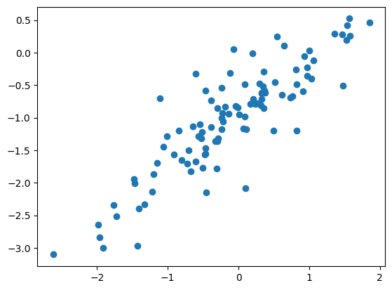
Indeed, most of the samples lie along the line, but a few of them go a bit farther away.
PyTorch fitting
Now let’s try fitting with several PyTorch optimizers and several step sizes to see the behavior. Note, that we would like to understand the behavior of the optimizer as a minimization algorithm, and not as a learning algorithm. Thus, there will be no division into train/validation/test. Instead, we will just see how well did we manage to minimize the desired loss on the training set we just sampled.
Our first ingredient is a loss for our stripped reformulation - something that takes an existing loss, multiplies by \(t\), and exponentiates it:
class StrippedTiltedLoss:
  def __init__(self, underlying_loss, t):
    super().__init__()
    self.underlying_loss = underlying_loss
    self.t = t

  def __call__(self, pred, target):
    return torch.exp(self.t * self.underlying_loss(pred, target))
Next, we shall write a function that fits a line to the data using a given loss and a given optimizer. It’s just a standard PyTorch training loop:
import torch

def pytorch_fit(x, y, criterion, make_optim_fn, n_epochs=100):
  # convert numpy arrays to torch tensors
  x = torch.as_tensor(x)
  y = torch.as_tensor(y)

  # define initial w to be the zero vector
  w_fit = torch.nn.Parameter(torch.zeros_like(x[0]))

  # create optimizer
  optim = make_optim_fn([w_fit])

  # regular PyTorch training loop.
  for epoch in range(n_epochs):
    for xi, yi in zip(x, y):
      pred = torch.dot(xi, w_fit)
      loss = criterion(pred, yi)

      optim.zero_grad()
      loss.backward()
      optim.step()

  return w_fit.detach()
To get a feeling, let’s try it the stripped tilted reformulation on top of the MSE loss:
from torch.nn import MSELoss

pytorch_fit(x, y,
            criterion=StrippedTiltedLoss(MSELoss(), t=1),
            make_optim_fn=lambda params: torch.optim.SGD(params, lr=1e-6))
The output I got is:
tensor([ 0.4708, -0.3032], dtype=torch.float64)
Doesn’t look like our line, so maybe we aren’t learning fast enough with such a small step size? Let’s try a larger step size:
pytorch_fit(x, y,
            criterion=StrippedTiltedLoss(MSELoss(), t=1),
            make_optim_fn=lambda params: torch.optim.SGD(params, lr=1e-4))
Now I got an output:
tensor([nan, nan], dtype=torch.float64)
We can add some printouts to understand what’s going on, but it’s quite simple. A large step size causes the weights to change sharply, which in turn causes large residuals, which in turn causes the gradients to become even more exponentially larger, causing even sharper changes to the learned weights.
We can conjecture, therefore, that there is a very narrow range of step sizes that perform reasonably well. A step size too small will make little progress, whereas a step size too large makes too much progress, causing exploding gradients. Consequently, hyper-parameter tuning becomes difficult and expensive, since pinpointing just the right step-size may require many training episodes, and waste previous time or money. Let’s verify our conjecture numerically, and plot the true tilted loss we obtain every step size.
Testing a set of step-sizes
Our first component is a function that computes the tilted loss for a given dataset. To ensure numerical accuracy and stability, I want to reuse PyTorch’s built-int logsumexp function. Using the fact that \(\frac{1}{n} = \exp(-\ln(n))\), we can reformulate the tilted loss as:
Now we can use logsumexp to compute the tilted loss without numerical issues:
import math

def compute_tilted_loss(w_fit, x, y, t):
  x = torch.as_tensor(x)
  y = torch.as_tensor(y)
  n = x.shape[0]
  squared_residuals = torch.square(x @ w_fit - y)
  return torch.logsumexp(t * squared_residuals - math.log(n), dim=-1) / t
Next, we write a function that experiments with our stripped equivalent of the tilted loss for various step-sizes with SGD:
from tqdm.auto import tqdm

def eval_sgd_exponential_loss(x, y, lrs, t=1):
  losses = []
  for lr in tqdm(lrs):
      optim_factory = partial(torch.optim.SGD, lr=lr)
      w_exp_fit = pytorch_fit(x, y, StrippedTiltedLoss(MSELoss(), t), optim_factory)
      w_exp_loss = compute_tilted_loss(w_exp_fit, x, y, t).item()
      losses.append(w_exp_loss)

  return losses
Let’s plot the results for a fine grid of step-sizes:
lrs = np.geomspace(1e-7, 1e-4, 60).tolist()
losses = eval_sgd_exponential_loss(x, y, lrs)

plt.plot(lrs, losses)
plt.xscale('log')
plt.yscale('log')
plt.xlim([np.min(lrs), np.max(lrs)])
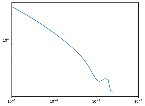
The x-axis is the step size, whereas the y-axis is the achieved value of the tilted loss. We can see that a tiny range, somewhere between \(10^{-5}\) and \(2 \times 10^{-5}\), results in a reasonable performance. Above that, we see that we’re have no data - that’s because the losses array contains NaNs. Our gradients exploded, and the optimizer failed for step sizes that are just a bit too large. Now let’s do some interesting tricks.
Trickery with logarithms
I do not recall exactly where, but in an exercise on convex optimization I encountered this simple fact:
\[\ln(z) = \min_v \{ z \exp(v) - v \} - 1\]The proof is a two liner - just take the derivative inside the \(\min\) w.r.t \(v\) and equate it with zero:
\[\begin{align*}\tag{V} &z \exp(v) - 1 = 0 \\ &v = -\ln(z) \end{align*}\]Substitute this \(v=-\ln(z)\) into the expression inside the \(\min\) to get the desired result. Remember this formula for \(v\) - it will be useful for PyTorch parameter initialization later in this post.
Writing a function as a minimum of a family of functions is called a variational formulation. So what we have is a variational formulation of the logarithm. Now let’s use it to do something useful. It’s a bit technical, but the end-result leads us in the right direction. We use the variational formulation of the logarithm in the tilted loss, and obtain the following:
\[\begin{aligned} \ln\left( \frac{1}{n} \sum_{i=1}^n \exp(t f(\mathbf{w}, \mathbf{x}_i)) \right) &= \min_v \left\{ \left( \frac{1}{n} \sum_{i=1}^n \exp(t f(\mathbf{w}, \mathbf{x}_i)) \right) \exp(v) - v \right\} - 1 \\ &= \min_v \left\{ \frac{1}{n} \sum_{i=1}^n \exp(t f(\mathbf{w}, \mathbf{x}_i) + v) - v \right\} - 1 \\ &= \min_v \left\{ \frac{1}{n} \sum_{i=1}^n \left( \exp(t f(\mathbf{w}, \mathbf{x}_i) + v) - v \right) \right\} - 1 \end{aligned}\]When minimizing, the constant \(-1\) at the end can also be stripped. Thus, training with a tilted loss amounts to solving the minimization problem
\[\min_{\mathbf{w}, v} \quad \frac{1}{n} \sum_{i=1}^n \left( \exp(t f(\mathbf{w}, \mathbf{x}_i) + v) - v \right)\]Let’s call this the variational formulation of the tilted loss. At first it appears we have not done anything useful - it’s again an average of exponentials. But a closer examination reveals that if \(v\) is negative it balances away large losses, and has a ‘stabilizing’ effect. So is it negative? Well, recalling equation \((V)\), the one I asked to remember, at the optimum we must have:
\[v = -\ln\left (\frac{1}{n} \sum_{i=1}^n \exp(t f(\mathbf{w}, \mathbf{x}_i)) \right )\]Except for extremely rare cases, losses are typically positive, their exponentials are at least 1, and therefore the argument of the logarithm is at least 1. This means that for any reasonable ML task, \(v\) at the optimum indeed is negative. But we do not care only about the optimum, we care about what happens throughout the entire training process. Thus, this variational formulation is just a heuristic which may, and we need to check weather it indeed does so.
An important component of making this heuristic useful is initializing \(v\) properly, so that the first epochs don’t fail on large gradients. But it’s not hard - the formula for \(v\) above is a great for initialization as well.
Testing our magic trick
Note, that we need to learn an additional parameter \(v\), which is conceptually not part of the model, but rather a part of the loss. Moreover, we will need a function to initialize our loss object, so that we can initialize \(v\). To facilitate the above, our losses will inherit torch.nn.Module, and will have an additional initialize method. Here is the stripped loss. Note that its initialization method does nothing:
class StrippedTiltedLoss(torch.nn.Module):
  def __init__(self, underlying_loss, t):
    super().__init__()
    self.underlying_loss = underlying_loss
    self.t = t

  def initialize(self, x, y):
    pass

  def forward(self, pred, target):
    exp_losses = torch.exp(self.t * self.underlying_loss(pred, target))
    return exp_losses.mean()
Here is the variational loss we just derived:
class VariationalTiltedLoss(torch.nn.Module):
  def __init__(self, t):
    super().__init__()
    self.t = t
    self.v = torch.nn.Parameter(torch.tensor(0.))

  def initialize(self, preds, targets):
    with torch.no_grad():
      init_losses = self.underlying_loss(preds, targets)
      n = init_losses.shape[0]

      v_init = -torch.logsumexp(self.t * init_losses - math.log(n), dim=-1)
      self.v.set_(v_init)

  def forward(self, pred, target):
    sample_loss = self.underlying_loss(pred, target)
    exp_tilted_losses = torch.exp(self.t * sample_loss + self.v) - self.v
    return exp_tilted_losses.mean()
It is assumed here that the underlying loss does not perform any reduction, such as averaging or summing the individual losses. We need the individual sample losses for our purposes, and thus we’re doing the averaging ourselves. In this post we train on individual samples, so no averaging is required, but in general people train on mini-batches of samples, and I wanted to make the code above re-usable in this scenario as well. This means that when passing the underlying loss, we need to tell it to avoid reducing, e.g. torch.nn.MSELoss(reduction='none')
To use losses that contain an addinal parameter, and to call the initialize method properly, we make a small modification to the fit_pytorch method we wrote above:
from itertools import chain

def pytorch_fit(x, y, criterion, make_optim, n_epochs=100):
  # convert numpy arrays to torch tensors
  x = torch.as_tensor(x)
  y = torch.as_tensor(y)
  dim = x.shape[1]
  dtype = x.dtype

  # perform proper initialization
  w_fit = torch.nn.Parameter(torch.zeros(dim, dtype=dtype))
  criterion.initialize(x @ w_fit, y)

  # create optimizer - don't foget that the `ciretion` now also has parameters!
  parameters_to_learn = chain(criterion.parameters(), [w_fit])
  optim = make_optim(parameters_to_learn)

  # regular PyTorch training loop.
  for epoch in range(n_epochs):
    for xi, yi in zip(x, y):
      pred = torch.dot(xi, w_fit)
      loss = criterion(pred, yi)

      optim.zero_grad()
      loss.backward()
      optim.step()

  return w_fit.detach()
Now let’s compare our two tilted loss formulations, the exponential, and the tilted exponential, in terms of their sensitivity to exactly pinpointing a narrow interval of step-sizes. We will expand our test a little bit, and try it for several values of the temperature \(t\) and two different optimizers - SGD and Adam. To that end, we wrote a function that tries both losses for a given set of temperatures, a set of learning rates, and a given optimizer. The results are gathered in a Pandas DataFrame.
from functools import partial
from itertools import product
import pandas as pd

def compare_tilted_formulations(x, y, ts, lrs, optim_ctor):
  records = []
  for t, lr in tqdm(list(product(ts, lrs))):
      make_optim_fn = partial(optim_ctor, lr=lr)

      mse_loss = MSELoss(reduction='none')
      w_exp_fit = pytorch_fit(x, y, StrippedTiltedLoss(mse_loss, t), make_optim_fn)
      w_tilted_fit = pytorch_fit(x, y, VariationalTiltedLoss(mse_loss, t), make_optim_fn)

      w_exp_loss = compute_tilted_loss(w_exp_fit, x, y, t).item()
      w_tilted_loss = compute_tilted_loss(w_tilted_fit, x, y, t).item()
      records.append(dict(t=t, lr=lr, loss_type='stripped', value=w_exp_loss))
      records.append(dict(t=t, lr=lr, loss_type='variational', value=w_tilted_loss))

  return pd.DataFrame.from_records(records)
Now let’s conduct our experiments. We begin with SGD:
lrs = np.geomspace(1e-7, 1e-4, 20).tolist()
ts = [0.25, 1, 2]
sgd_eval_recs = compare_tilted_formulations(x, y, ts=ts, lrs=lrs, optim_ctor=torch.optim.SGD)
To plot the results, it will be convenient to use seaborn:
import seaborn as sns
sns.set()

g = sns.relplot(data=sgd_eval_recs,
                hue='loss_type', col='t', x='lr', y='value', alpha=0.5)
g.set(xscale='log')
g.set(ylim=[0, 10])
g.set(yscale='asinh')
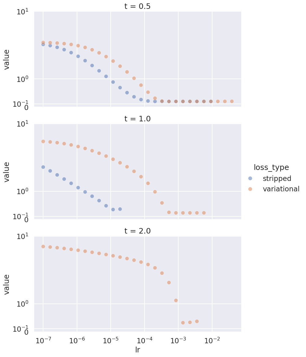
We see that \(t=0.5\) is not very challenging to both formulations. With \(t=1\) we already begin to see the difference - the stripped variant works well only for a very narrow interval, whereas the variational variant works in a significantly larger range. With \(t=2\), SGD fails altogether with the stripped variation.
But maybe SGD is less robust, so let’s try Adam:
adam_lrs = np.geomspace(1e-5, 1e2, 30)
adam_eval_recs = compare_tilted_formulations(x, y, ts=ts, lrs=adam_lrs, optim_ctor=torch.optim.Adam)

g = sns.relplot(data=adam_eval_recs,
                hue='loss_type', col='t', x='lr', y='value', alpha=0.5)
g.set(xscale='log')
g.set(ylim=[0, 20])
g.set(yscale='asinh')
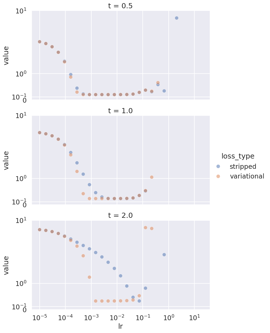
Indeed, Adam is more robust. It does not miserably fail for larger values of \(t\), but we can see a similar phenomenon. As \(t\) increases, it becomes harder to ‘pinpoint’ just the right step-size. So indeed, this simple trick may improve the computational cost of training a model with a tilted loss, and may significantly reduce the costs of training models when it’s to perform well not just on average, but also close to the worst case.
Summary
The variational formulation of the logarithm indeed helped, at least on the line fitting exercise. I do not wish to invest the resources required to try it out with a neural network, but I hope the code here is generic enough for you to try it out on your own ML task.
A variational formulation for the logarithm is nice, but we might have been able to do much better if we had a useful variational formulation for the entire LogSumExp function. I personally do not know if such a closed-form formulation exists, but if you do - talk to me, and let’s write a paper!
I would like to thank Prof. Tian Li and her collegues for their paper on tilted losses. It was enlightening, and I recommend you read it. And moreover, thank Prof. Bach for providing the inspiration.