Intro

Throughout this series, beginning here, we demonstrated various properties and applications of polynomial regression on different datasets. We used the Bernstein basis to demonstrate the importance of chosing a “good” polynomial basis, and that other well-known bases may be unfit for machine learning tasks. In this post, that concludes the series, we will try to understand why this happens by studying various regularization properties of the bases we encountered, including the standard power basis, the Chebyshev basis, the Legendre basis, and the Bernstein basis.

In this post we will not prove theorems, but rather demonstrate using an example. Therefore, there will be plenty of code and plots. And along the way we’ll learn some interesting tricks with linear regression and polynomials. All the code from this post is available in this notebook. So let’s get started!

The bias-variance tradeoff

When fitting data representing some “truth”, typically we observe a finite number of samples, and fit a model based on these samples. But what if, in theory, we did this again and again, and every time obtained a different set of samples? Well, our hope is that the corresponding models would, on average, be “close” to the truth.

Let’s simulate this by fitting a univariate function using polynomial regression. We will sample the function at some randomly chosen points, fit a polynomial, and repeat the experiment again and again.

Ingredients

Let’s write the components that will facilitate our experiments. We start by defining some interesting function \(f\) to approximate:

import numpy as np

def f(x):
  first = np.sin(np.pi * (x + np.abs(x - 0.75) ** 1.5))
  second = np.cos(0.8 * np.pi * (np.abs(x + 0.75) ** 1.5 - x)) + 0.5
  return 2 * np.minimum(first, second)

Seems like we have some weird parameters there. To see why, let’s see what \(f\) it looks like on \([-1, 1]\):

import matplotlib.pyplot as plt

plot_n = 10000
plot_xs = np.linspace(-1, 1, plot_n)

plt.plot(plot_xs, f(plot_xs))
plt.show()

bernstein_props_kink

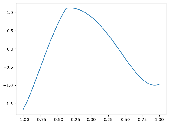
So I played a bit with the code in fn above until I got this interesting plot - \(f\) is composed of two functions joined at a “kink”. We will work with the interval \([-1, 1]\), since it’s easy to work with using NumPy’s built-in functions for polynomial bases.

To conduct our experiment, we will need a way to fit a polynomial using the basis of our choice by sampling some random points in \([-1, 1]\). Then, we would like to evaluate our polynomial on a dense grid of points in \([-1, 1]\) and compare it with the “truth”. To that end, we implemented a function that:

samples a set of points in \(\{ x_1, \dots, x_n \} \subseteq [-1, 1]\)
fits a polynomial \(p\) to \((x_1, f(x_1)), \dots, (x_n, f(x_n))\) of a given degree \(d\), using a given basis \(\mathbb{B}\), with a given L2 regularization coefficient \(\alpha\).
evaluates \(p\) at a given set of points.

Let’s see it’s code:

def fit_eval(vander_fn, eval_at, deg=20, n=40, reg_coef=0., ax=None, **plot_kws):
  # sample points for fitting
  xs = np.random.uniform(-1, 1, n)
  ys = f(xs)

  # build matrix and vector for least-squares regression
  vander_mat = vander_fn(xs, deg)
  if reg_coef > 0:
    coef_mat = np.identity(1 + deg) * np.sqrt(reg_coef)
    vander_mat = np.concatenate([vander_mat, coef_mat], axis=0)
    ys = np.concatenate([ys, np.zeros(1 + deg)], axis=-1)

  # compute polynomial coefficients
  coef = np.linalg.lstsq(vander_mat, ys, rcond=None)[0]

  # evaluate the polynomial at `eval_at`
  return vander_fn(eval_at, deg) @ coef

We can see by the default parameters that by default we sample 40 points, and fit a polynomial of degree 20. We will not change that throughout the post, but you are welcome to play with the notebook as you wish.

Note the code in the if reg_coef > 0 block in the function above. There is an interesting trick there for re-using existing NumPy libraries for least-squares regression, which are reliable and numerically stable, to solve a regularized least-squares problem. Note, that: \(\| A w - y\|^2 + \alpha \|w\|^2 = \sum_{j=1}^m ( a_j^T w - y_j )^2 + \sum_{i=1}^n (\sqrt{\alpha} w_i - 0)^2 = \left\| \begin{bmatrix} A \\ \sqrt{\alpha} I \end{bmatrix} w - \begin{bmatrix} y \\ 0 \end{bmatrix} \right\|^2\)

So, a regularized regression problem is reducible to a simple least-squares problem, with a data matrix padded by \(\sqrt{\alpha} I\), and the labels vector padded by zeros. That’s exactly what the code in the aforementioned block does. The reason I used this trick is to rely only on a small set of Python libraries, and avoid dependencies on scikit-learn and others.

So let’s see how it works:

ys = fit_eval(polyvander, plot_xs, deg=10)
plt.plot(plot_xs, ys, color='k')
plt.plot(plot_xs, fn(plot_xs), color='r')
plt.show()

poly_props_fit_eval_example

So doing it once, is nice, but we aim to repeat this experiment many times. So let’s write a function that does just that:

def fit_eval_samples(eval_at, vander_fn, n_iter=1000, **fit_eval_kwargs):
  y_samples = []
  for i in range(n_iter):
    ys = fit_eval(vander_fn, eval_at, **fit_eval_kwargs)
    y_samples.append(ys)
  y_samples = np.vstack(y_samples)
  y_true = f(eval_at)
  return y_samples, y_true

This function samples n_iter sets of points, computes n_iter least-squares fits, and evaluates each of the resulting polynomials at the points at the evaluation points eval_at. The results are organized into the rows of the matrix y_samples - the \(i\)-th row contains the values of the \(i\)-th polynomial. For convenience, it also computes the values of our “true” function \(f(x)\) at the evaluation points.

Finally, since we will be working on \([-1, 1]\), and the interval of approximation of the Bernstein basis is \([0, 1]\), let’s implement the Bernstein vandermonde function we already encountered, with appropriate scaling:

from scipy.stats import binom as binom_dist

def bernvander(x, deg, lb=-1, ub=1):
  x = np.array(x)
  x = np.clip((x - lb) / (ub - lb), lb, ub)
  return binom_dist.pmf(np.arange(1 + deg), deg, x.reshape(-1, 1))

Now that we have all our ingredients in place, let’s visualizee and analyze bias and variance.

Visualizing bias and variance

Let’s use our fit_eval_samples function to plot a large number of fits according to a given polynomial basis. Our function plots the fits and the true function returned by fit_eval_samples, and also the average polynomial, by averaging the returned y_samples array. Each one of the fit polynomials will be drawn in a transparent manner, so that we can see their density. And moreover, since badly fit polynomials “go crazy” near the boundaries, the function also accepts the y-axis limits for plotting.

def plot_basis_fits(n_iter, vander_fn, ylim=[-3, 3], alpha=0.1, ax=None, **fit_eval_kwargs):
  ax = ax or plt.gca()
  plot_xs = np.linspace(-1, 1, 10000)
  samples, y_true = fit_eval_samples(plot_xs, vander_fn, n_iter, **fit_eval_kwargs)
  mean_poly = np.mean(samples, axis=0)
  ax.plot(plot_xs, samples.T, 'r', alpha=alpha)
  ax.plot(plot_xs, mean_poly, color='blue', linewidth=2.)
  ax.plot(plot_xs, y_true, 'k--')
  ax.set_ylim(ylim)

Now we can use it to plot all our bases. The following function does just that by showing 100 different fit polynomials for every basis:

from numpy.polynomial.chebyshev import chebvander
from numpy.polynomial.legendre import legvander
from numpy.polynomial.polynomial import polyvander

def plot_all_bases(**plot_loop_kwargs):
  fig, axs = plt.subplots(2, 2, figsize=(10, 8))

  plot_basis_fits(100, polyvander, ax=axs[0, 0], **plot_loop_kwargs)
  axs[0, 0].set_title('Standard')

  plot_basis_fits(100, chebvander, ax=axs[0, 1], **plot_loop_kwargs)
  axs[0, 1].set_title('Chebyshev')

  plot_basis_fits(100, legvander, ax=axs[1, 0], **plot_loop_kwargs)
  axs[1, 0].set_title('Legendre')

  plot_basis_fits(100, bernvander, ax=axs[1, 1], **plot_loop_kwargs)
  axs[1, 1].set_title('Bernstein')

  plt.show()

Let’s let’s use it to visualize bias and variance without regularization:

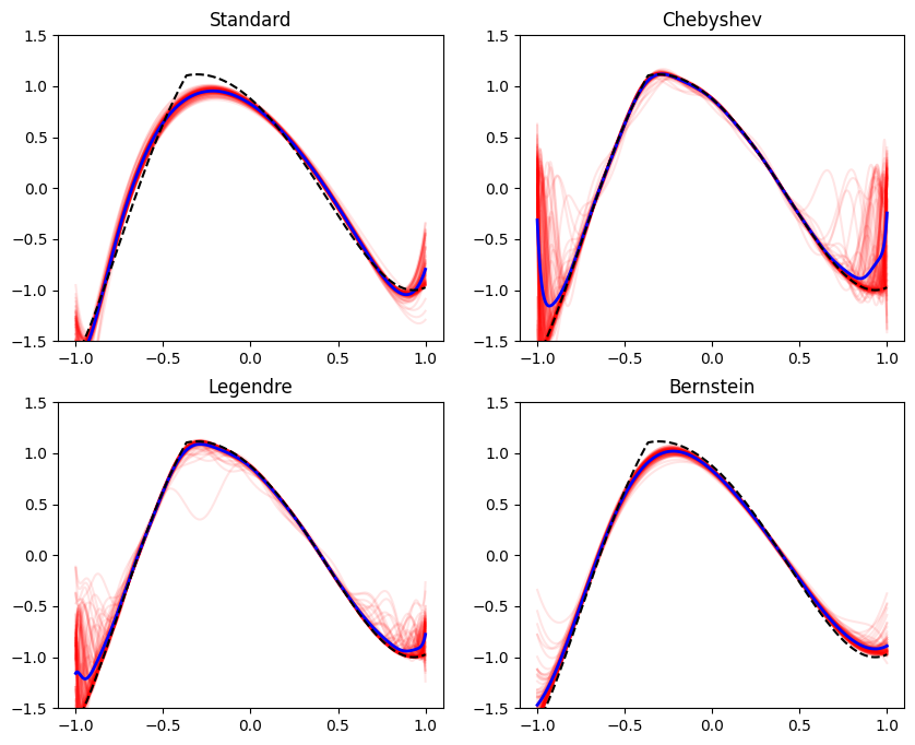
plot_all_bases(reg_coef=0.)

bases_bias_var_viz_0

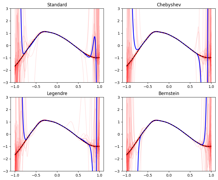
The dashed black line is the true function, the blue line is the average among the 100 polynomials, and the transparent red lines are the polynomials themselves. As expected, without regularization, the fit polynomials with all bases appear ‘crazy’. Moreover, even the average polynomial appears to be far away from the true function near the boundaries.

The difference between the average polynomial and the true function is called the bias, whereas the spread of the different polynomials around the average is called the variance. Of course, the bias and variance are different at every point. Near \(x=0\), they are pretty small, and as we approach the boundaries, both increase¹. The bias-variance tradeoff is a well-known concept in statistics, and a large body of research has been invested to its study. Here, we will try to approach it from a more empirical perspective.

Ideally, we would like both the bias and the variance to be small. A small bias means that on average over the samples, our polynomial represents the truth. A low variance means that regardless of the specific data-set, we will be always close to this truth, meaning that we will generalize well.

Typically, when measuring the bias, the deviation from the true function is squared. This is convenient, since the squared bias and the variance are a decomposition of the mean squared error. Informally, speaking:

\[\mathbb{E}[\mathrm{error}^2] = \mathbb{E}[\mathrm{bias}^2] + \mathrm{variance}\]

A more formal introduction can be found in the above-linked wikipedia article, and references therein.

Both bias and variance can be reduced either by a better estimation procedure or by more data. Let’s see what happens when we add more data - instead of using our default, and sampling 40 points for our least-squares regression, we will sample 200:

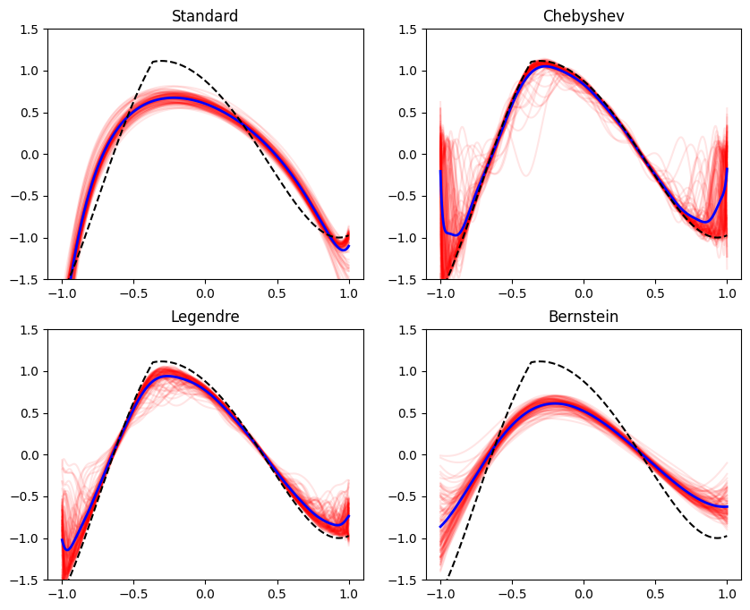
plot_all_bases(n=200, reg_coef=0.)

bases_bias_var_viz_0_n200

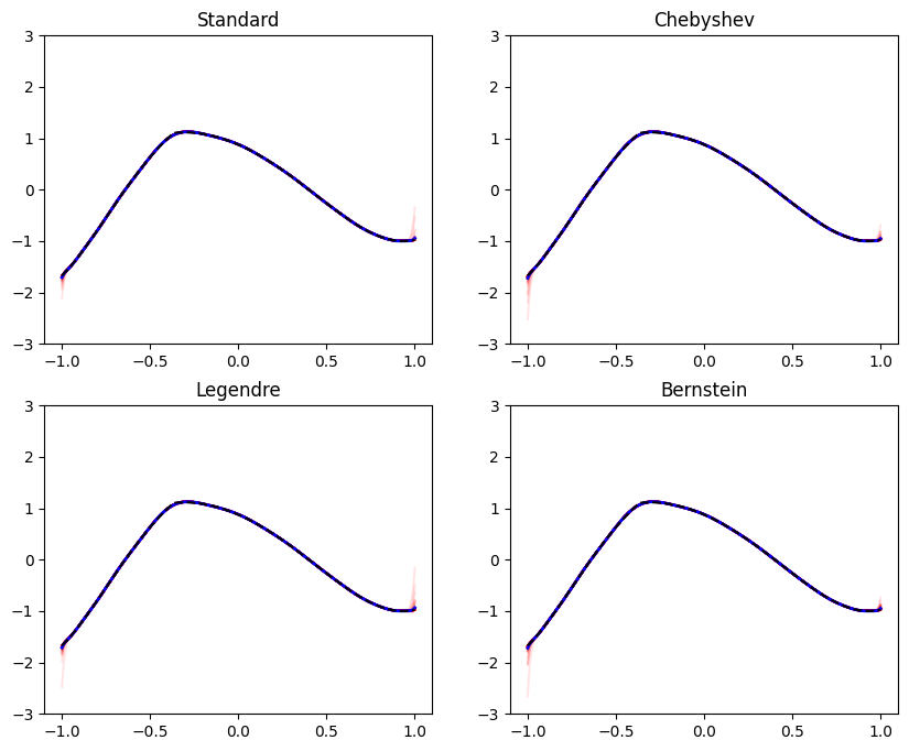
Appears much better! The mean polynomial almost coincides with the true function, and there’s little wiggling of individual polynomials around it. In this example, we have a very simlpe data-set with only one feature. In practice, data-sets are finite, and contain plenty of features. Not always enough to learn all coefficients in a model to the required precision.

As we pointed out, the bias-variance tradeoff also depends on the estimation procedure, and not only on the amount of data we have. Often in practice, our data-sets are finite, and we need to adapt the estimation procedure as well. Here we have two means to affect the estimation procedure - the choice of the basis, and the regularization coefficient. So let’s try using some regularization:

plot_all_bases(reg_coef=1e-3, ylim=[-1.5, 1.5])

bases_bias_var_viz_0.001

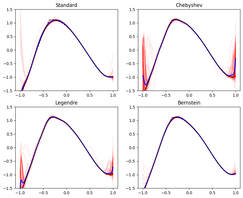
We can see that with this regularizaton coefficients, the Bernstein and the power basis behave much better, with the Bernstein basis being a bit better in terms of variance. It even looks close to what we can achieve with more data. But why the two other bases perform poorly? Maybe we’re under-regularizing the other two bases? Let’s try a larger coefficient:

plot_all_bases(reg_coef=1e-1, ylim=[-1.5, 1.5])

bases_bias_var_viz_0.1

We can clearly see we are over-regularizing the standard and the Bernstein bases - the average polynomial, the blue line, begins to get smoother and farther away from the true function. This is the expected increase of bias as a result of regularization. But the Chebyshev and Legendre bases are still a bit wiggly - so let’s try an even more aggressive regularization:

plot_all_bases(reg_coef=1, ylim=[-1.5, 1.5])

bases_bias_var_viz_1

It appears that these two bases do not improve with regularization - their bias increases, without a significant improvement improvement to the variance. So both components of the estimation procedure are crucial - the regularization and the basis.

Visualization is nice, but let’s measure these effects. We will try several regularization strengths, and for each strength - we will compute the average bias and variance we encounter among the evaluation points. Since both the bias and the variance vary along the interval \([-1, 1]\), we will average the squared bias and variance over the interval. Computing the mean squared bias and the variance for a given basis is straightforward:

def bias_variance_tradeoff(vander_fn, reg_coefs, nx=1000, **fit_eval_kwargs):
  xs = np.linspace(-1, 1, nx)
  biases = []
  vars = []
  for reg_coef in reg_coefs:
    y_samples, y_true = fit_eval_samples(xs, vander_fn, reg_coef=reg_coef, **fit_eval_kwargs)
    
    # mean squared bias over the samples, averaged over the interval [-1, 1]
    bias_agg = np.mean((np.mean(y_samples, axis=0) - y_true) ** 2)
    
    # variance over the samples, averaged over the interval [-1, 1]
    variance_agg = np.mean(np.var(y_samples, axis=0))
    
    biases.append(bias_agg)
    vars.append(variance_agg)

  return biases, vars

So now ler’s define regularization coefficients and conduct our experiment. It will be convenient to gather all the data to a Pandas dataframe, and plot it later:

import pandas as pd

reg_coefs = np.geomspace(1e-8, 1e2, 64)

biases, vars = bias_variance_tradeoff(polyvander, reg_coefs)
power_df = pd.DataFrame({'reg_coef': reg_coefs, 'bias': biases, 'variance': vars, 'basis': 'Power'})

biases, vars = bias_variance_tradeoff(chebvander, reg_coefs)
cheb_df = pd.DataFrame({'reg_coef': reg_coefs, 'bias': biases, 'variance': vars, 'basis': 'Chebyshev'})

biases, vars = bias_variance_tradeoff(legvander, reg_coefs)
leg_df = pd.DataFrame({'reg_coef': reg_coefs, 'bias': biases, 'variance': vars, 'basis': 'Legendre'})

biases, vars = bias_variance_tradeoff(bernvander, reg_coefs)
ber_df = pd.DataFrame({'reg_coef': reg_coefs, 'bias': biases, 'variance': vars, 'basis': 'Bernstein'})

all_df = pd.concat([power_df, cheb_df, leg_df, ber_df])

Let’s see a sample of our data-frame:

print(all_df)

Here is the result I got

        reg_coef      bias  variance      basis
 1.000000e-08  0.012936  4.517494      Power
 1.441220e-08  0.024666  1.617035      Power
 2.077114e-08  0.017855  2.934622      Power
 2.993577e-08  0.025465  1.882831      Power
 4.314402e-08  0.005049  2.150978      Power
..           ...       ...       ...        ...
2.317818e+01  0.594062  0.000286  Bernstein
3.340485e+01  0.614740  0.000133  Bernstein
4.814372e+01  0.629843  0.000076  Bernstein
6.938568e+01  0.640700  0.000036  Bernstein
1.000000e+02  0.648413  0.000018  Bernstein

[256 rows x 4 columns]

For every regularization coefficient and basis choice, we have a bias and a variance measurement. Let’s plot these using a SeaBorn scatterplot:

import seaborn as sns

to_plot = all_df.copy()
to_plot['size'] = np.log(to_plot['reg_coef'])

sns.scatterplot(data=to_plot, x='bias', y='variance', hue='basis', size='size')
ax = plt.gca()
ax.set_xscale('log')
ax.set_yscale('log')
ax.legend(bbox_to_anchor=(1.05,1), loc=2, borderaxespad=0.)
plt.show()

For each basis we have a different color, and the size of the points corresponds to the regularization coefficients, with larger points representing more aggressive regularization:

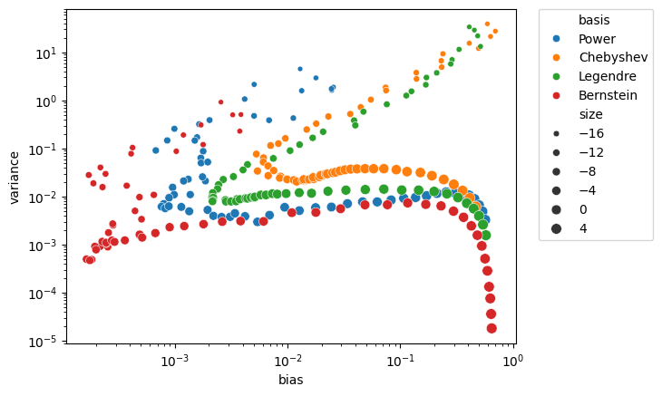
polynomial_bias_variance_tradeoff

Now we begin to understand the full picture. First, polynomials need regularization. A mild coefficient results in both a high measured bias and a high variance. At some point, we land on a nice trade-off curve. Moreover, we now see why the Bernstein basis was so successful in all our experiments before - it achieves a much better bias-variance tradeoff. Looking at the bottom-left part, we can see that it can achieve both low bias and low variance.

Does this phenomenon have a formal proof? Well, I wasn’t able to find one. But I was able to find a proof for a different sampling procedure, where the noise doesn’t come from sampling different data-sets, but from introducing noise in the \(y\) coordinate in this elaborate stackexchange answer. I suppose a similar proof could be derived for the case of a random data-set selection. I don’t believe I discovered something new here, but merely learned something that is “known” but was not formally published. If you have found something - please email me, and I will be glad to update the post and give a proper credit.

To summarize, we now understand that not only the class of models is important, but also its representation. Indeed class of polynomial functions can be represented with different bases, but some bases perform better than others for machine-learning tasks. So I think the most important lesson from this series is that:

We cannot judge a class of models on its own, without considering a concrete represention, since its performance is often tightly coupled to representation of choice.

Now let’s move to studying a different, but important theoretical property of the Bernstein basis.

Derivative sign regularization

Throughout this series we regularized the derivative of the polynomials to achieve a certain goal, either smoothness or monotonicity. I will concentrate on monotonicity, since it’s simpler to study. We in this post a theorem with an interesting consequence - if the coefficients of a polynomial in Bernstein form are monotone increasing, then the polynomial is monotone increasing. A similar result is obtained for a decreasing sequence.

But what about the inverse imlpication? Does every monotone-increasing polynomial also have a monotone-increasing coefficient sequence when represented according to the Bernstein basis? Well, the answer is NO. This means that when we fit a polynomial in the Bernstein basis with an increasing coefficients sequence, like we did in a previous post, we are not guaranteed to get the the best-fit increasing polynomial. There may be another increasing polynomial, whose Bernstein coefficients are not increasing, but it achieves a smaller training error.

So an interesting question begs to be answered - how far apart are increasing polynomials, and Bernstein polynomials with increasing coefficients? If this distance is small, the above fact should not bother us too much. But what if it is large? So let’s try to study this question empirically. This is not a formal proof, but rather a demonstration of some interesting phenomena.

What we will do is generate random increasing polynomials, and then try to find a least-squares fit to these polynomials using the Bernstein basis with increasing coefficients. So first we need to understand one important thing - how do we generate a polynomial that is guaranteed to be increasing on \([-1, 1]\). Having understood that, we will be able to write a simple Python function to generate some random increasing polynomial. Our plan is simple - we first learn how to generate a non-negative polynomial on \([-1, 1]\), and then compute its integral to obtain an increasing polynomial. To that end, let’s dive into century-old results on non-negative polynomials, initiated by no other than David Hilbert.

We begin by introducing the concept of a polynomial that is a sum of squares. A polynomial \(p(x)\) is a sum of squares if there exist polynomials \(q_1, \dots, q_m\) such that:

\[p(x) = q_1^2(x) + \dots + q_m^2(x)\]

Obiviously, any sum-of-squares polynomial is non-negative on the entire real-line. But we are not interested on the entire real-line, but on the interval \([-1, 1]\). It turns out that there exists a theorem for characterizing non-negative polynomials on this interval.

Theorem (Blekherman et. al. ², Theorem 3.72)

The polynomial \(p: \mathbb{R} \to \mathbb{R}\) of degree is non-negative on \([a, b]\) if and only if:

if the degree of \(p\) is the odd number \(2d+1\), then \(p(x) = (x - a) \cdot s(x) + (b-x) \cdot t(x)\) where \(s(x)\) and \(t(x)\) are sum of square polynomials of degree at most \(2d\).

if the degree of \(p\) is the even number \(2d\), then \(p(x) = s(x) + (x-a) \cdot (b-x) \cdot t(x)\) where \(s(x)\) and \(t(x)\) are sum of squares polynomials of degrees at most \(2 d\) and \(2 d - 2\).

So it appears that all we have to do is generate random two polynomials that are sums of squares, and construct \(p\) of the desired degree by multiplying and adding polynomials. To that end, we will use the np.polynomial.polynomial.Polynomial class that can represent operations such as addition and multiplication on arbitrary polynomials. So let’s implement the nonneg_on_biunit function, that generates a non-negative polynomial on the bi-unit interval \([-1, 1]\). To generate coefficients of the sum-of-squares polynomial, we will rely on the Cauchy distribution due to its heavy tails, so that we obtain a large variety of coefficients. Random numbers are generated by the np.random.standard_cauchy function.

from numpy.polynomial.polynomial import Polynomial

def sum_of_squares_poly(half_deg):
  num_coef = 1 + half_deg
  first_poly = Polynomial(np.random.standard_cauchy(num_coef))
  second_poly = Polynomial(np.random.standard_cauchy(num_coef))
  return first_poly * first_poly + second_poly * second_poly

def nonneg_on_biunit(deg):
  if deg == 0:
    return Polynomial(np.random.standard_cauchy()) ** 2
  if deg % 2 == 0: # odd degree
    s = sum_of_squares_poly(deg // 2)
    t = sum_of_squares_poly(deg // 2 - 1)
    return s + t * Polynomial(np.array([1, 0, -1]))
  else: # even degree
    s = sum_of_squares_poly((deg - 1) // 2)
    t = sum_of_squares_poly((deg - 1) // 2)
    return Polynomial(np.array([1, -1])) * s + \
           Polynomial(np.array([1, 1])) * t

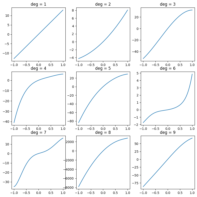
Does it work? Let’s see! We will plot randomly generated non-negative polynomials of various degrees:

np.random.seed(42)
fig, ax = plt.subplots(3, 3, figsize=(10, 10))
xs = np.linspace(-1, 1, 1000)
for deg, ax in enumerate(ax.flatten()):
  ys = nonneg_on_biunit(deg)(xs)
  ax.plot(xs, ys)
  ax.set_title(f'deg = {deg}')
plt.show()

nonneg_biunit_sample

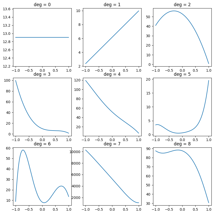
They indeed appear to be diverse, and non-negative. So let’s continue with our plan of creating increasing polynomials by integrating non-negative polynomials.

def increasing_on_biunit(deg):
  nonneg = nonneg_on_biunit(deg - 1)
  return nonneg.integ()

Let’s plot them, and see what we got:

np.random.seed(42)
fig, ax = plt.subplots(3, 3, figsize=(10, 10))
xs = np.linspace(-1, 1, 1000)
for deg, ax in enumerate(ax.flatten(), start=1):
  ys = increasing_on_biunit(deg)(xs)
  ax.plot(xs, ys)
  ax.set_title(f'deg = {deg}')
plt.show()

increasing_biunit_sample

Now, that our code appears to work, lets proceed to fitting Bernstein form polynomials with increasing coefficients to these increasing polynomials. First, for every degree, we will fit a Bernstein form polynomial of the same degree, to see if an increasing polynomial of degree \(d\) can be represented by a Bernstein polynomial of increasing coefficients of degree \(d\). To that end, we will use our beloved CVXPY package again, to constrain the Bernstein coefficients:

import cvxpy as cp

np.random.seed(42)
fig, ax = plt.subplots(4, 3, figsize=(10, 14))
xs = np.linspace(-1, 1, 1000)
for deg, ax in enumerate(ax.flatten(), start=1):
  true_ys = increasing_on_biunit(deg)(xs)

  vander_mat = bernvander(xs, deg)
  coef_var = cp.Variable(1 + deg)
  objective = cp.Minimize(cp.sum_squares(vander_mat @ coef_var - true_ys))
  prob = cp.Problem(objective, constraints=[cp.diff(coef_var) >= 0])
  prob.solve()

  coef = coef_var.value
  bern_ys = bernvander(xs, deg) @ coef

  ax.plot(xs, true_ys, 'k--')
  ax.plot(xs, bern_ys, 'r')
  ax.set_title(f'deg = {deg}')
plt.show()

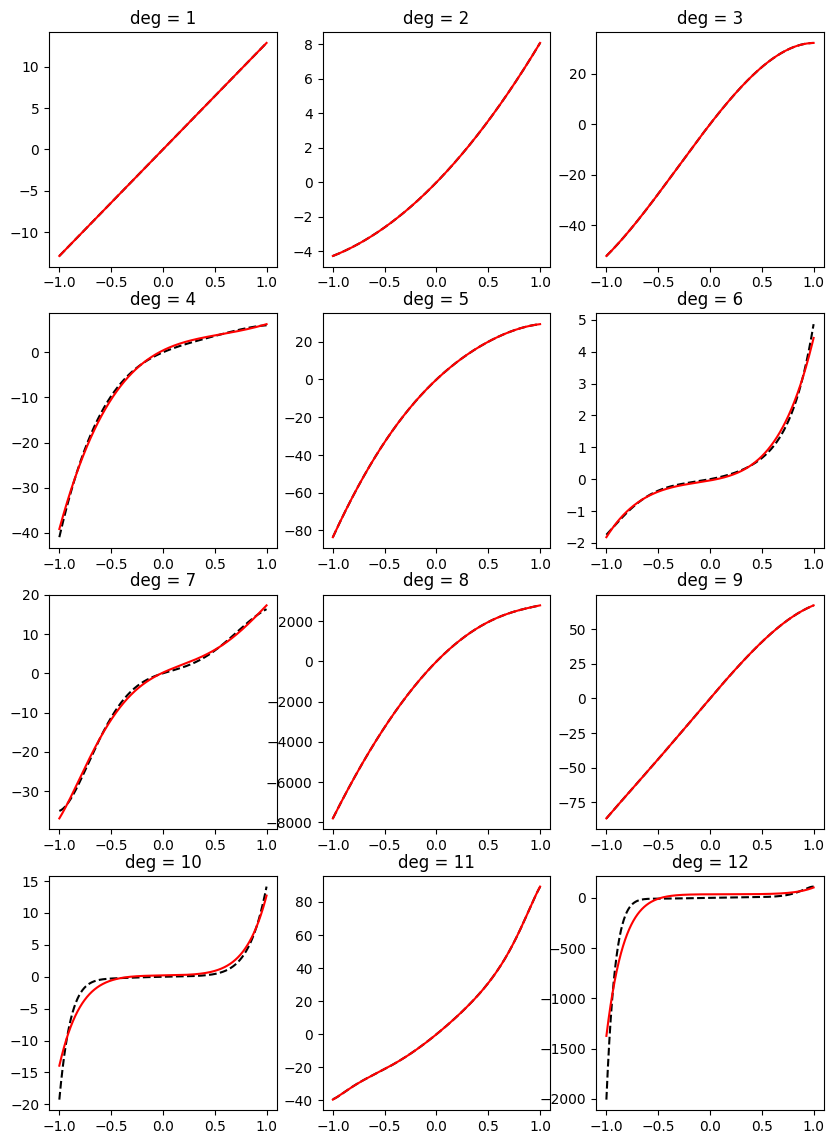
increasing_bernstein_samedegree_fit

We see that the fit is often very close, but doesn’t exactly match. Obivously, it is posisble to find an increasing polynomial of the corresponding degree to fit each function, since each function is itself a polynomial of that degree. But the constraint that the Bernstein coefficients increase reduces the space to a subset of increasing polynomials, and we are unable to exactly fit.

But what happens if we allow fitting Bernstein form polynomials of higher degrees? Say, for an increasing polynomial of degree d, we will fit a Bernstein polynomial with increasing coefficients of degree 2d. Maybe increasing the degree helps reduce the gap?

import cvxpy as cp

np.random.seed(42)
fig, ax = plt.subplots(4, 3, figsize=(10, 12))
xs = np.linspace(-1, 1, 1000)
for deg, ax in enumerate(ax.flatten(), start=1):
  true_ys = increasing_on_biunit(deg)(xs)

  fit_deg = 2 * deg  # <--- NOTE HERE
  vander_mat = bernvander(xs, fit_deg)
  coef_var = cp.Variable(1 + fit_deg)
  objective = cp.Minimize(cp.sum_squares(vander_mat @ coef_var - true_ys))
  prob = cp.Problem(objective, constraints=[cp.diff(coef_var) >= 0])
  prob.solve()

  coef = coef_var.value
  bern_ys = bernvander(xs, fit_deg) @ coef

  ax.plot(xs, true_ys, 'k--')
  ax.plot(xs, bern_ys, 'r')
  ax.set_title(f'deg = {deg}')
plt.show()

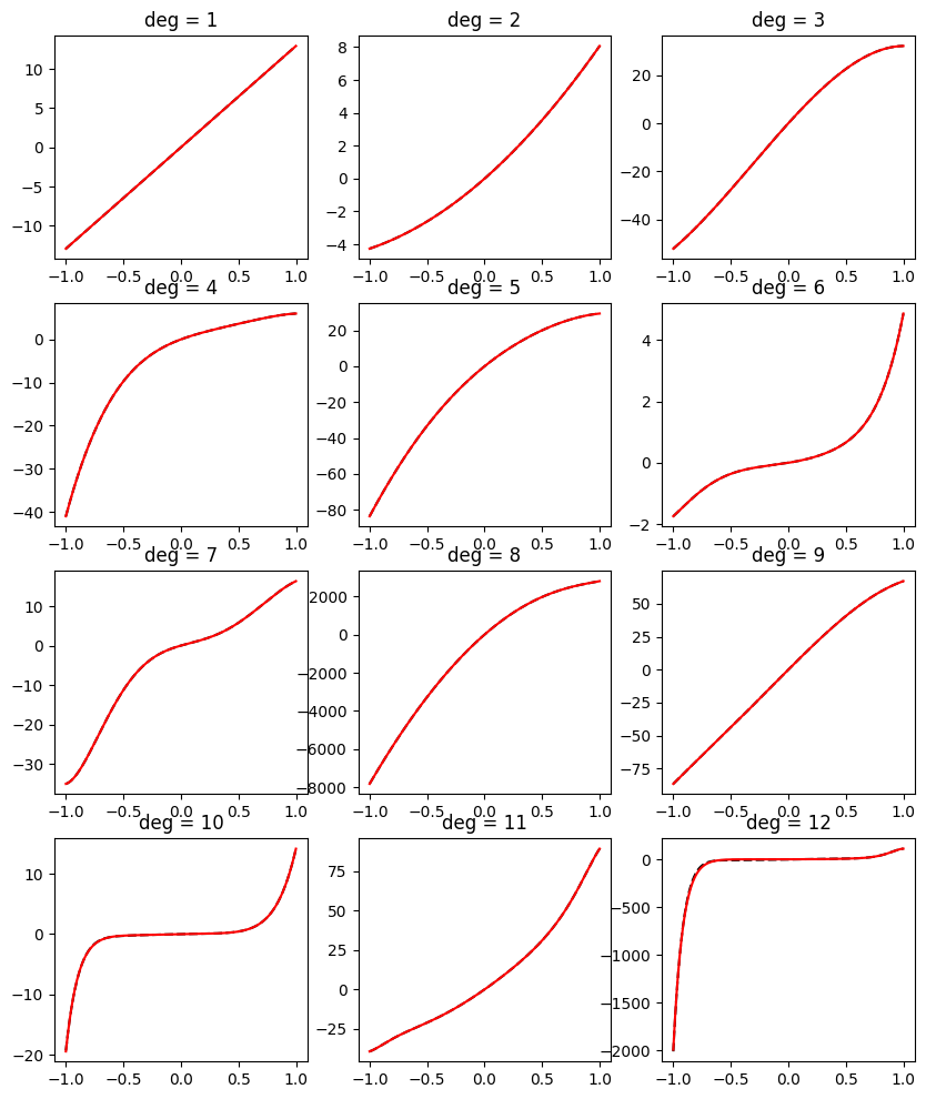
increasing_bernstein_twicedegree_fit

It appears it does. Empirically, we are able to fit increasing polynomials of degree d with polynomials of degree 2d with increasing Bernstein coefficients. In practice, this gap means that we may need to use a higher polynomial degree than we could, in theory, when fitting a polynomial to an increasing function.

Is a factor of two always sufficient to reduce the representation gap? If not - what is the relationship between the higher degree fit with increasing coefficients and the degree of the original polynomial? Personally, I don’t know. But it’s an interesting question. What is known is that among the bases that have direct shape control properties via their coefficients, which are colloquially known as “normalized totally-positive bases”, the Bernstein basis is the unique basis with “optimal” shape control properties. The meaning of the optimality criterion is out of the scope of this post, but I refer the readers to the paper Shape preserving representations and optimality of the Bernstein basis³ for reference. As we mentioned before, these properties are extensively used in computer graphics to represent curves and shapes, including all the text you are reading on the screen.

It is possible to use the minimal degree via semidefinite optimization by exploiting the theory of sum-of-squares polynomials, but this is out of the scope of this post. Moreover, the heavier computational burdain of semidefinite optimization typically makes this technique less applicable to fitting models to large amounts of data. Interested readers are referred to the book Semidefinite Optimization and Convex Algebraic Geometry².

Concluding remarks

This exploration of polynomial regression certainly taught me a lot. I learned that polynomials are not to be feared when designing regression models, when using a proper basis. The simplicity of polynomials is appealing - they have only one hyperparameter to tune, which is their degree. There are plenty of other function bases that can be used when fitting a nonlinear model using linear regression techniques, such as cubic splines, or radial basis functions. All of them are very useful, but they require more hyperparameter tuning, which may result in longer model fitting times and a slower model experimentation feedback loop. For example, splines, which are essentially piecewise polynomials with continuous (higher order) derivatives, require specifying their degree, the number of break-points, and the degree of derivative continuity. But given enough computational resources and data, these techniques probably perform better than polynomials.

I hope you enjoyed this series as much as I did, and the next posts will probably be on a different subject.

In theory, a least-squares estimator is unbiased. But it appears we don’t have enough samples so that our average polynomial approaches the true mean, and it appears as if we have bias. ↩
Grigoriy Blekherman, Pablo A. Parrilo, and Rekha R. Thomas. Semidefinite Optimization and Convex Algebraic Geometry. SIAM (2012). ↩ ↩²
J.M. Camicer and J.M. Pefia. Shape preserving representations and optimality of the Bernstein basis. Advances in Computational Mathematics 1 (1993) ↩