Shape restricted function models via polyhedral cones

Intro

In the previous post we learned a technique to use a neural network to produce the coefficients of a function in a basis of our choice. This “embedding vector” of coefficients can be regarded as a sequence of real numbers, whose shape affects the shape of the function the model represents. We wrote simple layers that can produce an increasing or a decreasing sequence of numbers - that was easy. But what about a convex sequence? Or a sequence that is both increasing and concave?

In this post we will dig deeper into how we can constrain the output of our embedding vectors to satisfy a family of constraints known as polyhedral constraints, that include the above use-cases. Then, after implementing a small PyTorch framework for the basic ideas presented here, we shall connect it to the previous post by fitting functions having interesting shape constraints.

The reason it’s a post and not a paper is, again, because the idea is not novel, and this post has been largely inspired by an idea introduced in an ECCV paper ¹ to solve a computer vision problem. Here we won’t be solving a computer vision problem, but fitting shape-constrained functions. The focus here is on applying the same idea for a different purpose, and demonstrating it on a concrete, tangible, and accessible use-case, with runnable code in a notebook you can deploy to Colab. So let’s get started!

Polyhedral sets

Consider the non-decreasing sequence

\[u_1 \leq u_2 \leq \dots \leq u_n.\]

The above is a compact way to write a system of linear inequalities:

\[\begin{align*} u_2 - u_1 &\geq 0 \\ u_3 - u_2 &\geq 0 \\ &\vdots \\ u_n - u_{n-1} &\geq 0 \end{align*}\]

The system can also be written in matrix form:

\[\underbrace{\begin{pmatrix} 1 & -1 & 0 & 0 & \dots & 0 \\ 0 & 1 & -1 & 0 & \dots & 0 \\ \vdots & & \ddots & \ddots & & \vdots \\ 0 & 0 & 0 & \dots & 1 & -1 \end{pmatrix}}_{\mathbf{A}} \underbrace{ \begin{pmatrix} u_1 \\ \vdots \\ \vdots \\ u_n \end{pmatrix}}_{\mathbf{u}} \geq \begin{pmatrix} 0 \\ \vdots \\ 0 \end{pmatrix}\]

It turns out sets of all vectors \(\mathbf{u}\) satisfying constraints of the above form have been extensively studied. They are called polyhedral cones. So let’s get formally introduced: for a matrix \(\mathbf{A}\), consider the set \(C(\mathbf{A})\) defined by:

\[C(\mathbf{A}) = \left\{ \mathbf{u} : \mathbf{A} \mathbf{u} \geq \mathbf{0} \right\}\]

Let’s decrypt the name polyhedral cone. Why polyhedral? A polyhedron, in mathematics, is a high dimensional generalisation of what we know as a polygon: it’s something that has ‘vertices’, or other forms of ‘sharp boundaries’. We will indeed soon see that such sets do have such sharp boundaries. Why cones? It’s also a generalisation of what we know as a 2D or a 3D cone - a set of infinite rays, as depicted below:

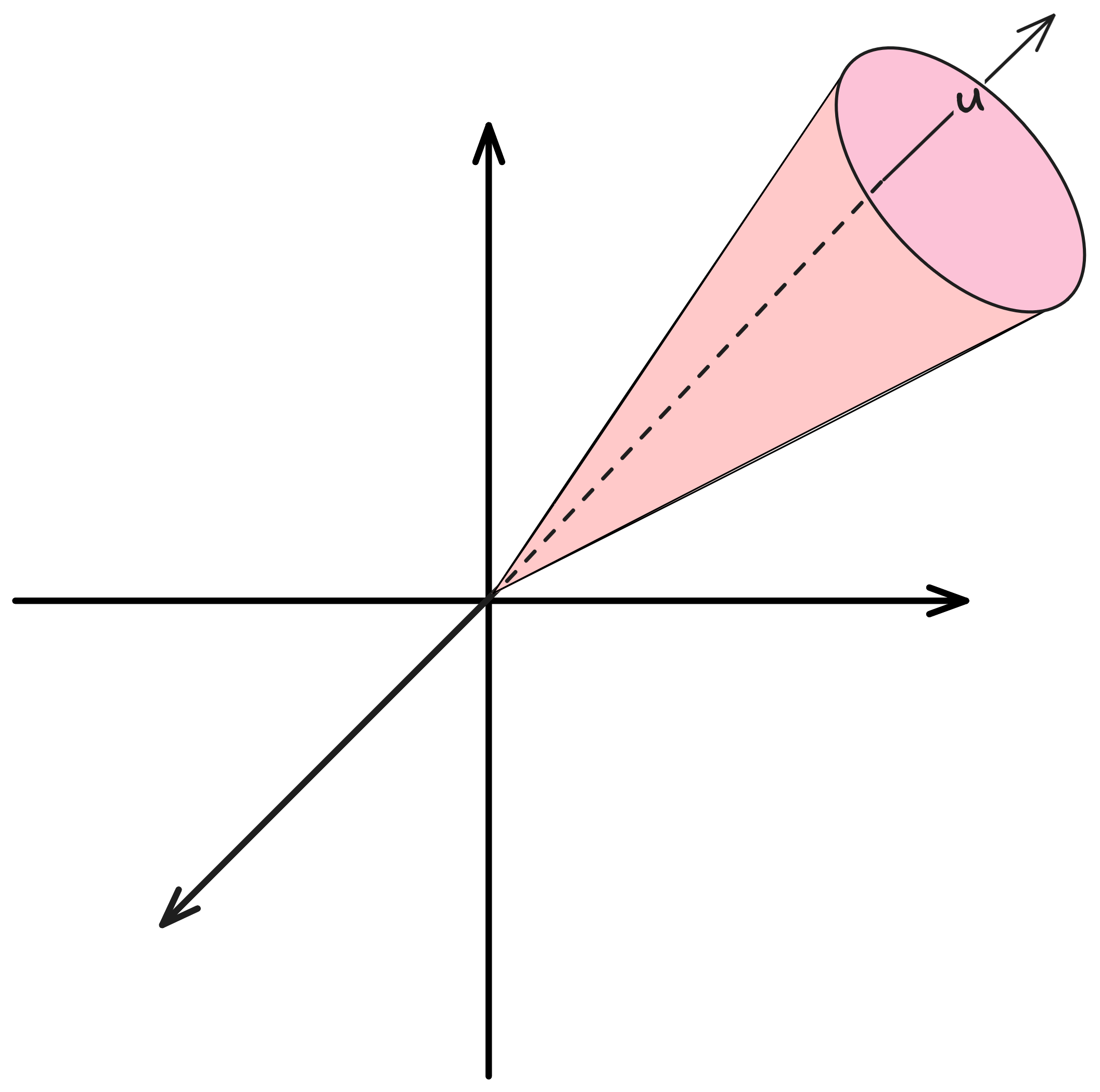
Mathematically, a cone is a set such that if \(\mathbf{u}\) is in the set, then also \(\lambda \mathbf{u}\) is in the set for any \(\lambda \geq 0\). This means that any vector \(\mathbf{u}\) in the cone signifies a direction of a ray belonging to the cone. In a sense, a cone is defined by the set its rays. Our set \(C(\mathbf{A})\) is indeed a cone, since if the inequality \(\mathbf{A} \mathbf{u} \geq 0\) is satisfied by some vector \(\mathbf{u}\), then it’s satisfied by any non-negative multiple of \(\mathbf{u}\).

It turns out that non-decreasing, non-increasing, convex, or concave constraints are all polyhedral conic constraints, since they can be written as linear inequalities with a zero on the right-hand side. We saw non-decreasing constraints above. What about convexity? Well, we just need to require the discrete analogue of the second derivative to be non-negative:

\[u_{i-1} - 2 u_i + u_{i+1} \geq 0 \qquad \forall i = 2, \dots, n-1.\]

Concavity is similar - the discrete analogue of the second derivative is non-positive, or equivalently, its negation is non-negative:

\[-u_{i-1} + 2 u_i - u_{i-1} \geq 0 \qquad \forall i = 2, \dots, n - 2.\]

But what makes polyhedral cones special and useful in machine learning? It’s the following version of the Weyl-Minkowski theorem²³ for polyhedral cones :

There is \(\mathbf{A} \in \mathbb{R}^{m \times n}\) such that \(C = \{ \mathbf{u} : \mathbf{A} \mathbf{u} \geq 0 \}\) if and only there are vectors \(\mathbf{r}_1, \dots, \dots, \mathbf{r}_p\) such that \(C = \{ t_1 \mathbf{r}_1 + \dots + t_p \mathbf{r}_p :t_i \geq 0 \}\)

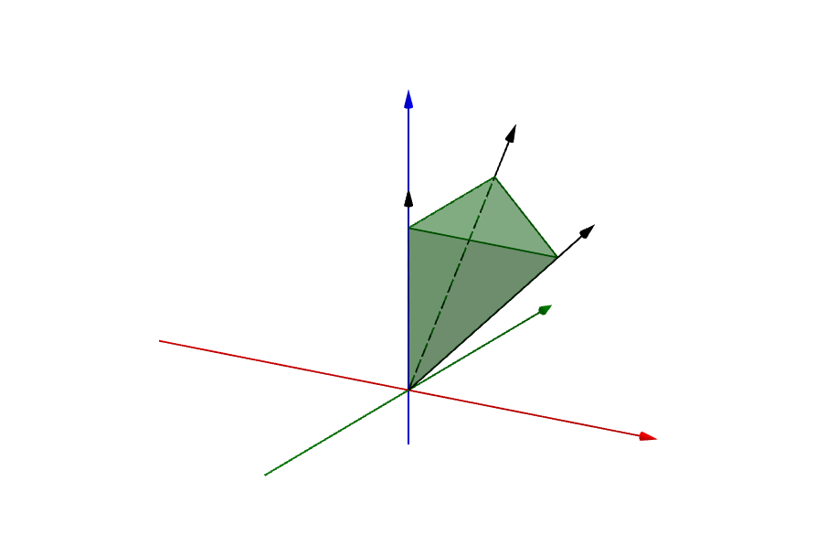
Namely, a polyhedral cone can be represented either by linear inequalities with a zero right-hand side, or by a linear combination with non-negative coefficients \(\mathbf{u} = t_1 \mathbf{r}_1 + \dots + t_p \mathbf{r}_p\). The vectors \(\mathbf{r}_1, \dots, \mathbf{r}_p\) are called the generators or extremal rays of the set. Generators, because they are used to generate any point in the set. Extremal, because these are exactly the “sharp boundaries” of \(C(\mathbf{A})\), as depicted below. The black vectors are the extremal rays of the green cone (source: Wikipedia):

To make things more concise, we can embed the generators into the columns of the matrix \(\mathbf{R}\), and write:

\[\mathbf{u} = \mathbf{R} \mathbf{t}\]

The theorem ensures that for every \(\mathbf{A}\) representing the inequalities, we have a corresponding \(\mathbf{R}\) representing the generator rays, and vice versa.

But why an ML practitioner would be interested in this result? A machine-learned model can easily produce a non-negative vector \(\mathbf{t}\) using known activation functions, such as ReLU or SoftPlus. Then, we can use a linear layer with matrix \(\mathbf{R}\) to compute a vector \(\mathbf{R} \mathbf{t}\) in our desired cone. Therefore, a concatenation of a non-negativity layer and a linear layer with an appropriate matrix can be thought of as a “polyhedral cone” layer: it generates vectors that lie in a polyhedral cone of our choice. This is illustrated below:

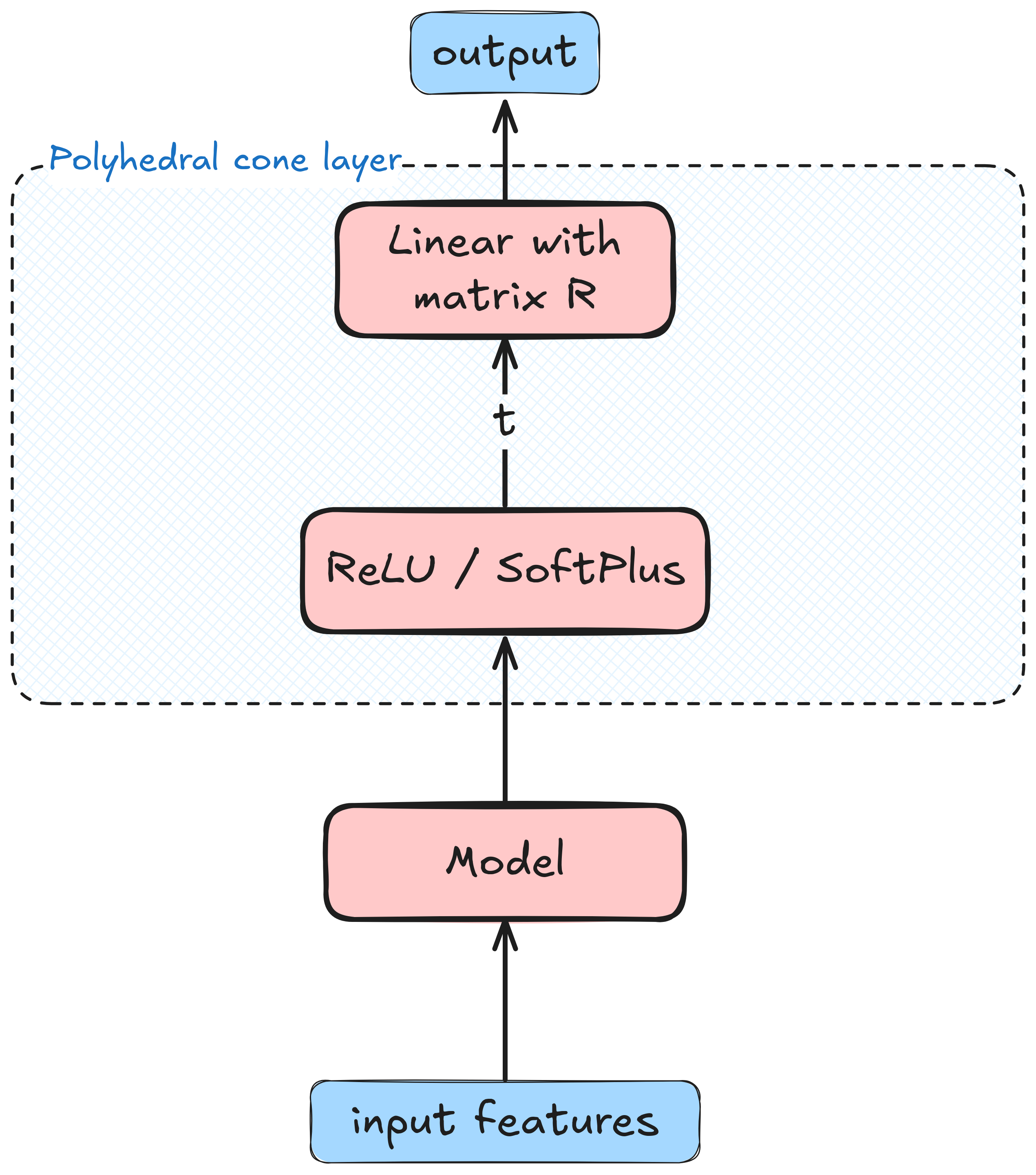
Note, that in this case \(\mathbf{R}\) is not learned, but rather is a constant matrix specifically designed to generate the cone we need. So the reason polyhedral cones are useful in ML is because we can make sure that our neural network produces vectors that lie in the cone, by design, using elementary tools that every ML practitioner knows: ReLU activations and linear layers!

To end our discussion of the generator ray representation, we note that we can have two generators that are just the negation of each other, i.e \(\mathbf{r}_i = -\mathbf{r}_j\). For example, consider the matrix:

\[\mathbf{R} = \begin{pmatrix} 1 & -1 & 3 \\ 2 & -2 & -2 \\ 3 & -3 & 0 \end{pmatrix}\]

Its first two columns are just negations of each other. This matrix represents a cone that is generated by

\[\begin{align*} \mathbf{R} \mathbf{t} &= t_1 \cdot \begin{pmatrix}1 \\ 2 \\ 3 \end{pmatrix} + t_2 \cdot \begin{pmatrix}-1 \\ -2 \\ -3 \end{pmatrix} + t_3 \cdot \begin{pmatrix} 3 \\ -2 \\ 0 \end{pmatrix} \\ &= (t_1 - t_2)\cdot \begin{pmatrix}1 \\ 2 \\ 3\end{pmatrix} + t_3 \cdot \begin{pmatrix}3 \\ -2 \\ 0 \end{pmatrix} \end{align*}\]

for any \(t_1, t_2, t_3 \geq 0\). Since \(t_1 - t_2\) can be any real number, positive or negative - two columns having opposite signs can just be ‘shrunk’ into one column, whose coefficient does not have to be non-negative. \(t_3\), of course, remains non-negative.

So in practice, when we are given a matrix \(\mathbf{R}\) of generators for our cone, we should be also have corresponding instructions regarding each component of \(\mathbf{t}\) - is it non-negative, or arbitrary. This little details seems like a complication, but we shall soon see that the contrary is true. The components which do not have to be non-negative will be referred to as the linear components. Those that have to be non-negative are the conic components.

Now let’s implement our ‘polyhedral cone layer’, as depicted in the illustration above. Since not all generator coefficients have to be non-negative, we shall first implement a ‘masked activation’ layer, that applies an activation function only to a subset of the components denoted by a mask. It’s a bit intricate - since we need to somehow apply activation to a subset of the components of our input vector, and keep the remaining components unchanged. We achieve it with the help of the torch.masked_scatter function - it’s a bit advanced, but it works. Finally, it shall be easier to use this class by specifying the mask of the components for which we do not apply the activation. So here it is:

import torch
from torch import nn

class MaskedActivation(nn.Module):
  def __init__(self, mask=None, activation=nn.ReLU):
    """
    Applies activation to (potentially) a subset of the input components. 
    Args:
      mask: The mask of coordinates to which we should NOT apply the activation.
        `None` means applying the activation to all components. It is assumed
        that `mask` is a 1D tensor, that applies to the last dimension of the input
      activation: The activation to apply.
    """
    super().__init__()
    self.activation = activation()
    self.register_buffer('mask', mask)
  
  def forward(self, x):
    if self.mask is None:
      return self.activation(x) 
    else:
      activated = self.activation(x[..., ~self.mask])
      result = x.masked_scatter(~self.mask, activated)
      return result

To represent our generators, we shall also need a helper function to create a linear layer with constant (or frozen) weight matrix:

def frozen_linear(weights):
  in_dim, out_dim = weights.shape
  layer = nn.Linear(in_dim, out_dim, bias=False)
  layer.weight = nn.Parameter(weights, requires_grad=False)
  return layer

And now we can create our polyhedral cone layer - a concatenation of our activation with our generators:

def polyhedral_cone_module(generators, linear_mask=None, nonneg_activation=nn.ReLU):
  generators = generators / torch.linalg.vector_norm(generators, dim=0, keepdim=True)
  return nn.Sequential(
  	MaskedActivation(linear_mask, nonneg_activation),
    frozen_linear(generators)
  )

This is where it’s obvious why our MaskedActivation layer accepts a mask telling it where to avoid applying the activation - this is exactly the linear mask. You may also have noticed that the first line in the function above does something strange - it normalizes the columns of the generator matrix. But why? Well, in practice, algorithms for training ML models like ‘nice’ normalized data and ‘nice’ normalized matrices. Since the generators only denote the direction of the cone’s rays, their length does not change the cone they generate. I’ll save you the time spent on first writing this entire blog post without the normalization step, encountering the numerical issues, and then adding it in to solve numerical issues. So I added this step in the first place.

Now let’s try out our generic polyhedral cone module for non-decreasing sequences. For that, we will need to represent non-decreasing sequences using a generator matrix \(\mathbf{R}\). Luckily, it’s quite simple to do manually. As we saw in the last post, a nondecreasing sequence can be created by specifying its first compoenent by an arbitrary number \(t_1\), and adding to it non-negative numbers \(t_2, d_3, \dots, t_{n} \geq 0\) sequentially to produce the next elements:

\[\begin{pmatrix}u_1 \\ u_2 \\ u_3 \\ \vdots \\ u_n\end{pmatrix} = \begin{pmatrix}t_1 \\ t_1 + t_2 \\ t_1+t_2+t_3 \\ \vdots \\ t_1 + \dots + t_n \end{pmatrix} = \underbrace{\begin{pmatrix} 1 & 0 & 0 & \dots & 0 \\ 1 & 1 & 0 & \dots & 0 \\ 1 & 1 & 1 & \dots & 0 \\ \vdots & \vdots & \vdots & \ddots & \vdots \\ 1 & 1 & 1 & \dots & 1 \end{pmatrix}}_{\mathbf{R}} \begin{pmatrix} t_1 \\ t_2 \\ \vdots \\ t_n \end{pmatrix}\]

We can do it, alternatively, by specifying the last component by an arbitrary number \(t_n\), and subtracting non-negative numbers ‘backwards’ to generate the non-decreasing sequence: \(\begin{pmatrix} u_1 \\ u_2 \\ \dots \\ u_n \end{pmatrix} = \begin{pmatrix} t_n - t_{n - 1} - \dots - t_2 - t_1 \\ \vdots \\ t_n - t_{n-1} \\ t_n \end{pmatrix} = \begin{pmatrix} -1 & -1 & -1 & \dots & -1 & 1 \\ 0 & -1 & -1 & \dots & -1 & 1 \\ & \vdots & & \ddots & \vdots & \vdots \\ 0 & 0 & \dots & 0 & -1 & 1 \\ 0 & 0 & \dots & 0 & 0 & 1 \end{pmatrix} \begin{pmatrix}t_1 \\ t_2 \\ \vdots \\ t_n \end{pmatrix}\)

This demonstrates that the representation with generators does not have to be unique.

Now let’s construct a PyTorch module that produces non-decreasing matrix using our polyhedral_cone_module function. Here, we shall use the first matrix \(\mathbb{R}\) - the upper triangular matrix of ones. Note, that since \(t_1\) is a ‘linear’ coefficient, meaning it doesn’t have to be non-negative, so we shall also use the appropriate mask :

def nondecreasing_module(n):
  generators = torch.tril(torch.ones(n, n)) # the matrix of ones under the diagonal
  linear_mask = torch.zeros(n, dtype=bool)
  linear_mask[0] = 1
  return polyhedral_cone_module(generators, linear_mask)

Let’s try it out, and use our module to create some non-decreasing vectors:

n = 8
mod = nondecreasing_module(n)

torch.manual_seed(42)
print(mod(torch.randn(n)))
print(mod(torch.randn(n)))
print(mod(torch.randn(n)))

tensor([0.3367, 1.0963, 1.9135, 2.7285, 3.0102, 3.6145, 5.9269, 6.3511])
tensor([0.4617, 1.2974, 2.2933, 3.4709, 4.8660, 5.0353, 5.3516, 6.6343])
tensor([1.3221, 2.5051, 2.8869, 3.2736, 4.8561, 5.9502, 6.4929, 7.6605])

They do appear non-decreasing! So now that we have the machinery working, let’s look for a more generic way to derive the matrix \(\mathbf{R}\) that corresponds to a desired polyhedral cone. But we have two obstacles.

The first obstacle is of a combinatorial nature - to represent an \(n\)-dimensional polyhedral cone, we may need more than \(2^n\) generator rays in the worst case. This is a consequence of the McMullen theorem⁴. This means that even for a small dimension \(n\), we might have a matrix \(\mathbf{R}\) that has more columns than the number of the atoms in the entire universe. Fortunately, the polyhedral cones in this post to not suffer from this exponential explosion of generator rays. We just saw an example with the increasing cone - the matrix \(\mathbf{R}\) had exactly \(n\) columns.

The second challenge is practical - how do we compute the generator rays of the cone we desire? Do we have a convenient Python library to which we feed the inequalities we want, and it gives us the corresponding matrix \(\mathbf{R}\)? For non-decreasing sequences we could derive it ourselves, but it may be non-trivial in general. As ML practitioners, we just want to write PyTorch layers - we don’t want to deal with computational polyhedral geometry. It turns out we do have such a library, and that’s exactly what we shall explore in the next section.

Computing generator matrices

There are two prominent parallel streams of research on algorithms for translating between the generator and the inequality representations of polyhedral cones. One is a family of algorithms based on the so-called Reverse Search Method⁵, whereas the other is based on the so-called Double Description method⁶. It’s important to acknowledge both, but in this post we shall use the double-description method, because it’s accessible from a simple Python library. So we will not dive into the algorithms, but rather use the library. After all, as ML researchers, we prefer using the results developed by the talented polyhedral geometry researchers, over doing polyhedral geometry research ourselves.

So there is a C library, cddlib, that was written by Komei Fukua. Its source code can be found on GitHub. He is also the author of an interesting open access book on polyhedral computation, which is available here. It turns out his library also has a nice Python wrapper - pycddlib. So let’s install it in our Colab notebook:

%pip install pycddlib-standalone

Now we can import and use it in our notebook. So let’s describe a polyhedral cone representing increasing sequences, and then use this example to explain the format the pycddlib library expects its input to be in:

import numpy as np
import cdd

def make_cdd_cone(A):
  """Creates a libcdd polyhedral cone given the matrix describing the inequalities A x ≥ 0. """
  # define the RHS of the inequalities. In our case - everything is ≥ 0
  b = np.zeros((A.shape[0], 1))

  # the library operates assuming we describe inequalities in the form:
  #    b + A x ≥ 0
  # and expects b and A to be concatenated into one big matrix.
  Ab = np.hstack([b, A])

  # create and print the polyhedral cone object
  mat = cdd.matrix_from_array(Ab, rep_type=cdd.RepType.INEQUALITY)
  poly = cdd.polyhedron_from_matrix(mat)
  return poly

# polyhedral cone for non-decreasing sequences:
cone = make_cdd_cone(np.array(
    [[-1,  1,  0,  0,  0,  0,  0,  0],
     [ 0, -1,  1,  0,  0,  0,  0,  0],
     [ 0,  0, -1,  1,  0,  0,  0,  0],
     [ 0,  0,  0, -1,  1,  0,  0,  0],
     [ 0,  0,  0,  0, -1,  1,  0,  0],
     [ 0,  0,  0,  0,  0, -1,  1,  0],
     [ 0,  0,  0,  0,  0,  0, -1,  1]]))
print(cone)

Here is the output:

begin
 7 9 real
  0 -1  1  0  0  0  0  0  0
  0  0 -1  1  0  0  0  0  0
  0  0  0 -1  1  0  0  0  0
  0  0  0  0 -1  1  0  0  0
  0  0  0  0  0 -1  1  0  0
  0  0  0  0  0  0 -1  1  0
  0  0  0  0  0  0  0 -1  1
end

The line 7 9 real means that our cone is defined by 7 inequalities, and each inequality is described by 9 numbers. And indeed, below we have a matrix of 7 rows, each having 9 numbers. The first column of the matrix is all zeros, whereas the other columns are exactly the matrix \(\mathbf{A}\). At this stage, we can think of the first column as the right-hand side of the inequalities, which is zero.

Now this is where the library is useful - it lets is convert inequality form to generator form! So let’s do it:

generators = cdd.copy_generators(cone)
print(generators)

Here is the output:

V-representation
linearity 1  8
begin
 8 9 real
  0 -1  0  0  0  0  0  0  0
  0 -1 -1  0  0  0  0  0  0
  0 -1 -1 -1  0  0  0  0  0
  0 -1 -1 -1 -1  0  0  0  0
  0 -1 -1 -1 -1 -1  0  0  0
  0 -1 -1 -1 -1 -1 -1  0  0
  0 -1 -1 -1 -1 -1 -1 -1  0
  0  1  1  1  1  1  1  1  1
end

The first line, V-represenation, means that our set is in the generators form, as opposed to the inequality form. The second line, linearity 1 8 means we have one “linear” generator, and it’s the \(8^{\mathrm{th}}\) generator. Note, that in the printout, the indices begin from 1, rather than from 0. Then, we have a matrix of generators, again, with a column of zeros. The zero column has a special mathematical meaning, which here we shall interpret as ‘these are generators of a cone’. Now here is an important detail - in contrast to the mathematical convention in this post, generators are in the rows, rather than the columns of the matrix. To convert this matrix to our desired form, we need to transpose it.

The generators object above also has a array property with the generators, and the lin_set property specifying the set of linear generators. So let’s create a convenience function to print the generators in the columns of a matrix, together with the set of linear generators:

def print_generators(cone):
  generators = cdd.copy_generators(cone)
  print('Linear generators: ', generators.lin_set)
  print('Generator matrix: ')
  gen_mat = np.array(generators.array)
  gen_mat = gen_mat[:, 1:] # discard the first column of zeros
  gen_mat = gen_mat.T
  print(gen_mat)

print_generators(cone)

Linear generators:  {7}
Generator matrix: 
[[-1. -1. -1. -1. -1. -1. -1.  1.]
 [ 0. -1. -1. -1. -1. -1. -1.  1.]
 [ 0.  0. -1. -1. -1. -1. -1.  1.]
 [ 0.  0.  0. -1. -1. -1. -1.  1.]
 [ 0.  0.  0.  0. -1. -1. -1.  1.]
 [ 0.  0.  0.  0.  0. -1. -1.  1.]
 [ 0.  0.  0.  0.  0.  0. -1.  1.]
 [ 0.  0.  0.  0.  0.  0.  0.  1.]]

Indeed, it’s one of the two matrices \(\mathbf{R}\) we manually obtained for non-decreasing sequences. Note, that in the lin_set property, the linear indices are zero-based. But now we can see that the process does not have to be manual - it can be automated.

What about a non-increasing sequence? Well, we could derive it ourselves easily, but why bother? Let’s do it ourselves:

# print generators for non-increasing sequences
# note - the matrix is exactly the negated matrix of non-decreasing sequences
# we used above.
cone = print_generators(make_cdd_cone(np.array(
    [[1,  -1,  0,  0,  0,  0,  0,  0],
     [ 0, 1,  -1,  0,  0,  0,  0,  0],
     [ 0,  0, 1,  -1,  0,  0,  0,  0],
     [ 0,  0,  0, 1,  -1,  0,  0,  0],
     [ 0,  0,  0,  0, 1,  -1,  0,  0],
     [ 0,  0,  0,  0,  0, 1,  -1,  0],
     [ 0,  0,  0,  0,  0,  0, 1,  -1]])))

Linear generators:  {7}
Generator matrix: 
[[1. 1. 1. 1. 1. 1. 1. 1.]
 [0. 1. 1. 1. 1. 1. 1. 1.]
 [0. 0. 1. 1. 1. 1. 1. 1.]
 [0. 0. 0. 1. 1. 1. 1. 1.]
 [0. 0. 0. 0. 1. 1. 1. 1.]
 [0. 0. 0. 0. 0. 1. 1. 1.]
 [0. 0. 0. 0. 0. 0. 1. 1.]
 [0. 0. 0. 0. 0. 0. 0. 1.]]

Well, we can see the pattern, right? It’s just an upper-triangular matrix of ones. So we can also implement a corresponding PyTorch layer:

def nonincreasing_module(n):
  generators = torch.triu(torch.ones(n, n))

  linear_mask = torch.zeros(n, dtype=bool)
  linear_mask[n-1] = True # the last generator is linear

  return polyhedral_cone_module(generators, linear_mask)

Let’s see if it works:

n = 8
mod = nonincreasing_module(n)

torch.manual_seed(42)
print(mod(torch.randn(n)))
print(mod(torch.randn(n)))
print(mod(torch.randn(n)))

tensor([ 1.2874,  0.9507,  0.8596,  0.7242,  0.6091,  0.6091,  0.6091, -0.2256])
tensor([2.1994, 1.7378, 1.5487, 1.2399, 0.8352, 0.3387, 0.3387, 0.3387])
tensor([3.0661, 1.7440, 1.1661, 1.1661, 1.1661, 0.5613, 0.2811, 0.2811])

Appears to be working! What about convex sequences? For that, we will require the second-order differences of the sequence to be non-negative:

\[u_{i + 1} - 2 u_i + u_{i-1} \geq 0, \qquad i = 1, \dots, n-1\]

So let’s compute the generator form and see the pattern:

# print generators for a convex sequence
cone = print_generators(make_cdd_cone(np.array(
    [[1,  -2,  1,  0,  0,  0,  0,  0],
     [ 0, 1,  -2,  1,  0,  0,  0,  0],
     [ 0,  0, 1,  -2,  1,  0,  0,  0],
     [ 0,  0,  0, 1,  -2,  1,  0,  0],
     [ 0,  0,  0,  0, 1,  -2,  1,  0],
     [ 0,  0,  0,  0,  0, 1,  -2,  1]])))

Linear generators:  {6, 7}
Generator matrix: 
[[ 1.  2.  3.  4.  5.  6.  7. -6.]
 [ 0.  1.  2.  3.  4.  5.  6. -5.]
 [ 0.  0.  1.  2.  3.  4.  5. -4.]
 [ 0.  0.  0.  1.  2.  3.  4. -3.]
 [ 0.  0.  0.  0.  1.  2.  3. -2.]
 [ 0.  0.  0.  0.  0.  1.  2. -1.]
 [ 0.  0.  0.  0.  0.  0.  1.  0.]
 [ 0.  0.  0.  0.  0.  0.  0.  1.]]

It takes a few seconds to see the pattern, but it’s not hard. The generator matrix is divided into four blocks:

\[\left( \begin{array}{ccccc|c} 1 & 2 & 3 & \dots & n - 1 & -(n - 2) \\ 0 & 1 & 2 & \dots & n - 2 & -(n - 3) \\ \vdots & \ddots & \ddots & 1 & 2 & -1 \\ 0 & 0 & \dots & 0 & 1 & 0 \\ \hline 0 & 0 & \dots & 0 & 0 & 1 \end{array} \right)\]

The top-left block is an upper-triangular matrix of simple progressions from 1 to \(n - k\). The bottom-left block is a row of zeros. The top-right block is a decreasing column from \(-(n-2)\) to zero, and the bottom-right block is the scalar 1. Beyond the block structure, we see that the last two generators, indexed 6,7, are the linear generators. So let’s implement a function that creates such a generator matrix:

def make_convex_generators(n):
  top_left = torch.cumsum(torch.triu(torch.ones((n - 1, n - 1))), dim=1)
  top_right = torch.arange(-(n-2), 1).reshape(-1, 1)
  top = torch.cat([top_left, top_right], dim=1)

  bottom_left = torch.zeros((1, n - 1))
  bottom_right = torch.ones((1, 1))
  bottom = torch.cat([bottom_left, bottom_right], dim=1)

  generators = torch.cat([top, bottom], dim=0)
  return generators

make_convex_generators(8)

tensor([[ 1.,  2.,  3.,  4.,  5.,  6.,  7., -6.],
        [ 0.,  1.,  2.,  3.,  4.,  5.,  6., -5.],
        [ 0.,  0.,  1.,  2.,  3.,  4.,  5., -4.],
        [ 0.,  0.,  0.,  1.,  2.,  3.,  4., -3.],
        [ 0.,  0.,  0.,  0.,  1.,  2.,  3., -2.],
        [ 0.,  0.,  0.,  0.,  0.,  1.,  2., -1.],
        [ 0.,  0.,  0.,  0.,  0.,  0.,  1.,  0.],
        [ 0.,  0.,  0.,  0.,  0.,  0.,  0.,  1.]])

Appears to work! So now let’s implement our PyTorch module:

def convex_module(n):
  generators = make_convex_generators(n)
  linear_mask = torch.zeros(n, dtype=bool)
  linear_mask[-2:] = True
  return polyhedral_cone_module(generators, linear_mask)

Now let’s test it. Since convexity is easier to see visually, we will plot the resulting sequences to see if they’re indeed convex:

import matplotlib.pyplot as plt

n = 32
layer = convex_module(n)

torch.manual_seed(56)
for i in range(6):
  t = torch.randn(n)
  plt.plot(layer(t))
plt.show()

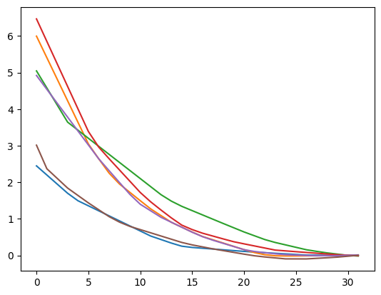
They indeed appear all convex, but something look suspicious! Why are they all almost the same? Maybe our cddlib library does not compute the right generators for entire space the convex sequences, but only for a small subset? It turns out what we see is a result of our use of normally distributed random inputs to our layer. This specific distribution of vectors indeed produces a very specific distribution of convex sequences. But we can get interesting sequences with different inputs, for example:

t = (torch.linspace(-1, 1, n)).square()
t[-1] = n / 2
t[-2] = -n / 2
plt.plot(layer(t))

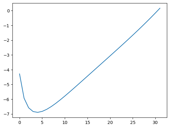
Indeed looks very different. This means that any model that uses our layer to generate convex sequences will have to learn to provide those ‘interesting’ input vectors \(\mathbf{t}\) as the input to our layer, so that the output of our layer is the correct one.

Concave sequences are extremely similar, the inequality is just the negation of the convexity inequality:

\[-u_{i-1} + 2 u_i - u_{i+1} \geq 0, \qquad i = 2, \dots, n - 1\]

Let’s ask the cddlib library to create a generator matrix for us:

# print generators for a convex sequence
cone = print_generators(make_cdd_cone(np.array(
    [[-1,  2,  -1,  0,  0,  0,  0,  0],
     [ 0, -1,  2,  -1,  0,  0,  0,  0],
     [ 0,  0, -1,  2,  -1,  0,  0,  0],
     [ 0,  0,  0, -1,  2,  -1,  0,  0],
     [ 0,  0,  0,  0, -1,  2,  -1,  0],
     [ 0,  0,  0,  0,  0, -1,  2,  -1]])))

Linear generators:  {6, 7}
Generator matrix: 
[[-1. -2. -3. -4. -5. -6.  7. -6.]
 [ 0. -1. -2. -3. -4. -5.  6. -5.]
 [ 0.  0. -1. -2. -3. -4.  5. -4.]
 [ 0.  0.  0. -1. -2. -3.  4. -3.]
 [ 0.  0.  0.  0. -1. -2.  3. -2.]
 [ 0.  0.  0.  0.  0. -1.  2. -1.]
 [ 0.  0.  0.  0.  0.  0.  1.  0.]
 [ 0.  0.  0.  0.  0.  0.  0.  1.]]

The pattern appears similar to the convex sequences, but the structure of the blocks is a bit different. And here too the last two generators are linear. It’s not hard to figure out that the following code produces this matrix directly with PyTorch:

def make_concave_generators(n):
  top_left = torch.cumsum(torch.triu(torch.ones((n - 1, n - 1))), dim=1)
  top_right = torch.arange(-(n-2), 1).reshape(-1, 1)
  top = torch.cat([top_left, top_right], dim=1)

  bottom_left = torch.zeros((1, n - 1))
  bottom_right = torch.ones((1, 1))
  bottom = torch.cat([bottom_left, bottom_right], dim=1)

  mat = torch.cat([top, bottom], dim=0)
  mat[:n-2, :n-2] *= -1
  return mat

make_concave_generators(8)

tensor([[-1., -2., -3., -4., -5., -6.,  7., -6.],
        [-0., -1., -2., -3., -4., -5.,  6., -5.],
        [-0., -0., -1., -2., -3., -4.,  5., -4.],
        [-0., -0., -0., -1., -2., -3.,  4., -3.],
        [-0., -0., -0., -0., -1., -2.,  3., -2.],
        [-0., -0., -0., -0., -0., -1.,  2., -1.],
        [ 0.,  0.,  0.,  0.,  0.,  0.,  1.,  0.],
        [ 0.,  0.,  0.,  0.,  0.,  0.,  0.,  1.]])

Now we can implement and try out the concave module:

def concave_module(n):
  generators = make_concave_generators(n)
  linear_mask = torch.zeros(n, dtype=bool)
  linear_mask[-2:] = True
  return polyhedral_cone_module(generators, linear_mask)

n = 32
layer = concave_module(n)

torch.manual_seed(42)
for i in range(10):
  t = torch.randn(n)
  plt.plot(layer(t))
plt.show()

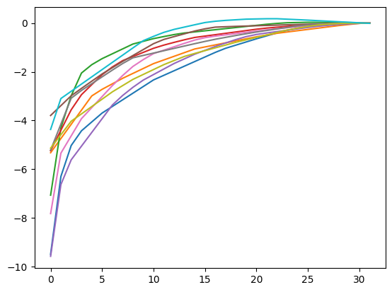
Indeed all look concave!

So what if we want a concave and non-decreasing function? Easy peasy! Need to satisfy both the types of inequalities:

\[\begin{align*} -u_{i-1} + 2 u_i - u_{i+1} \geq 0 & \qquad i = 2, \dots, n - 1 \\ u_{i+1} - u_i \geq 0 & \qquad i = 1, \dots, n - 1 \end{align*}\]

So we just concatenate the two inequality matrices we saw above, one after the other, and ask cddlib to make the appropriate generator matrix:

# print generators for concave non-decreasing sequences
print_generators(make_cdd_cone(np.array(
    [[-1,  2,  -1,  0,  0,  0,  0,  0],
     [ 0, -1,  2,  -1,  0,  0,  0,  0],
     [ 0,  0, -1,  2,  -1,  0,  0,  0],
     [ 0,  0,  0, -1,  2,  -1,  0,  0],
     [ 0,  0,  0,  0, -1,  2,  -1,  0],
     [ 0,  0,  0,  0,  0, -1,  2,  -1],
     [-1,  1,  0,  0,  0,  0,  0,   0],
     [ 0, -1,  1,  0,  0,  0,  0,   0],
     [ 0,  0, -1,  1,  0,  0,  0,   0],
     [ 0,  0,  0, -1,  1,  0,  0,   0],
     [ 0,  0,  0,  0, -1,  1,  0,   0],
     [ 0,  0,  0,  0,  0, -1,  1,   0],
     [ 0,  0,  0,  0,  0,  0, -1,   1]]
    )))

Linear generators:  {7}
Generator matrix: 
[[-7. -6. -5. -4. -3. -2. -1.  1.]
 [-6. -5. -4. -3. -2. -1.  0.  1.]
 [-5. -4. -3. -2. -1.  0.  0.  1.]
 [-4. -3. -2. -1.  0.  0.  0.  1.]
 [-3. -2. -1.  0.  0.  0.  0.  1.]
 [-2. -1.  0.  0.  0.  0.  0.  1.]
 [-1.  0.  0.  0.  0.  0.  0.  1.]
 [ 0.  0.  0.  0.  0.  0.  0.  1.]]

The pattern is quite simple - a triangular block of decreasing integers, concatenated to a column of ones. And only the last generator is linear. The following PyTorch code generates such a matrix:

def concave_nondecreasing_generators(n):
  generators = -torch.ones(n, n).triu(1).cumsum(dim=1).fliplr()
  generators[:, -1] = torch.ones(n)
  return generators

concave_nondecreasing_generators(8)

tensor([[-7., -6., -5., -4., -3., -2., -1.,  1.],
        [-6., -5., -4., -3., -2., -1., -0.,  1.],
        [-5., -4., -3., -2., -1., -0., -0.,  1.],
        [-4., -3., -2., -1., -0., -0., -0.,  1.],
        [-3., -2., -1., -0., -0., -0., -0.,  1.],
        [-2., -1., -0., -0., -0., -0., -0.,  1.],
        [-1., -0., -0., -0., -0., -0., -0.,  1.],
        [-0., -0., -0., -0., -0., -0., -0.,  1.]])

Here is our concave-nondecreasing layer:

def concave_nondecreasing_cone_module(n):
  generators = concave_nondecreasing_generators(n)
  linear_mask = torch.zeros(n, dtype=bool)
  linear_mask[-1] = True
  return polyhedral_cone_module(generators, linear_mask)

Let’s try it out with a few random inputs:

n = 32
layer = concave_nondecreasing_cone_module(n)

torch.manual_seed(42)
for i in range(10):
  t = torch.randn(n)
  plt.plot(layer(t))
plt.show()

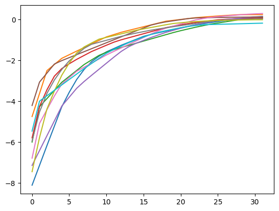
Beautiful! Devising the generator matrix for concave and non-decreasing sequences ourselves is not so trivial this time. We may have devised the right generator matrix after thinking about it. I can speak for myself here, but for me it would take a very long time of ‘thinking about it’ until I would come up with the correct set of generators. The algorithms implemented in thecddlib library automate this process, and produce provably correct generator matrix and linear set.

So now we have an interesting method to constrain the output of a model to lie in our desired polyhedral cone:

1. Feed cddlib with the appropriate inequalities, and let it create the generators and the linear set
2. Implement PyTorch code that produces the same generator matrix
3. Feed the generator matrix to polyhedral_cone_module to produce a PyTorch layer that transforms arbitrary vectors into vectors that provably lie in the cone we desire.

Now let’s combine this with our shape-constrained polynomial functions from the last post, to fit a model that produces shape-constrained functions.

Example - fitting concave functions

Now let’s remind ourselves why we wanted to constrain the output vector of a neural network to satisfy conic constraints. The reason is because we want to use such vectors as coefficients of a Bernsten polynomial, that inherits the properties of its coefficients, such as monotonicity, or convexity. We continue the adventure we started in the previous post of fitting increasing, decreasing, convex, or concave functions using neural networks!

So let’s re-use the BernsteinPolynomialModel class from the previous post, that represents a function \(f(\mathbf{x}, z)\) with a given constraint on the shape of the function, as a function of \(z\). For completeness, I repeat its definition here:

class BernsteinPolynomialModel(nn.Module):
  def __init__(self, x_model, coef_transformer):
    super().__init__()
    self.x_model = x_model
    self.coef_transformer = coef_transformer

  def forward(self, x, z):
    coefs = self.coef_transformer(self.x_model(x))
    degree = coefs.shape[-1] - 1
    basis = bernstein_basis(degree, z)
    return torch.sum(coefs * basis, dim=-1)

The restriction of shape comes from the coef_transformer sub-module, that produces the right shape-constrained coefficients for the Bernstein polynomial basis. Here, we shall use the concave_module we just implemented using our polyhedral cone library to make sure that our module fits concave functions of \(z\).

For the demo, we shall generate a synthetic data-set using the following funciton:

import numpy as np

def np_softplus(x):
  return np.log1p(np.exp(x))

def hairy_concave_func(x, z):
  x1, x2, x3 = x[..., 0], x[..., 1], x[..., 2]
  return np_softplus(x1) * np.sqrt(0.05 + z) - np_softplus(x3) * (z - np.cos(x2) ** 2) ** 2

Looking at it as a function of \(z\), we can see that it is of the form \(a \sqrt{0.05 + z} - b(z - c)^2\). It’s indeed concave: square roots are concave, and a ‘sad’ parabola is also concave. Let’s plot a few examples for various inputs \(\mathbf{x}\):

zs = np.linspace(0, 1, 1000)
plt.plot(zs, hairy_concave_func(np.array([-1, 0.1, 0.5]), zs), label='function 1')
plt.plot(zs, hairy_concave_func(np.array([1, 0.5, -0.5]), zs), label='function 2')
plt.plot(zs, hairy_concave_func(np.array([-1.5, 0.8, 0.1]), zs), label='function 3')
plt.legend()
plt.show()

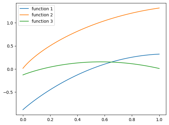
To generate an entire data-set based on this function, we adopt a similar approach to the previous post - we generate random features \((\mathbf{x}, z)\), and generate labels using \(f(\mathbf{x}, z) + \varepsilon\), where \(\varepsilon\) is normally distributed noise, and \(f\) is our hairy concave function above:

def generate_dataset(n_rows, noise=0.02, mean=0, std=1):
  xs = std * np.random.randn(n_rows, 3) + mean
  zs = np.random.rand(n_rows)
  labels = hairy_concave_func(xs, zs) + np.random.randn(n_rows) * noise

  xs = torch.as_tensor(xs).to(dtype=torch.float32)
  zs = torch.as_tensor(zs).to(dtype=torch.float32)
  labels = torch.as_tensor(labels).to(dtype=torch.float32)
  if torch.cuda.is_available():
    xs = xs.cuda()
    zs = zs.cuda()
    labels = labels.cuda()

  return xs, zs, labels

Now, similarly to the previous post, we shall generate train and validation set iterators:

from batch_iter import BatchIter

batch_size = 256
train_iter = BatchIter(*generate_dataset(50000), batch_size=batch_size)
valid_iter = BatchIter(*generate_dataset(10000), batch_size=batch_size)

We shall also modify the make_model function from the previous post, to create a model with concave rather than increasing constraints:

def make_model(layer_dims, constrained=True):
  # create a fully connected ReLU network
  layers = [
      layer
      for in_dim, out_dim in zip(layer_dims[:-1], layer_dims[1:])
      for layer in [nn.Linear(in_dim, out_dim), nn.ReLU()]
  ]

  if constrained:
    # define a model for x
    x_model = nn.Sequential(*layers[:-1])

    # construct a network for predicting non-decreasing functions
    # the polynomial degree is the output dimension of the last
    # layer.
    return BernsteinPolynomialModel(
        x_model,
        concave_module(layer_dims[-1]) # <-- CONCAVE CONSTRAINTS
    )
  else:
    layers.append(nn.Linear(layer_dims[-1], 1))
    return nn.Sequential(*layers)

Note, that the function above can create both a concavely-constrained model using our concave_module as the component that produces Bernstein coefficients, and a fully unconstrained model, by using a regular fully-connected layer instead of Bernstein polynomials.

Now let’s train it. To that end, we will reuse the functions train_model, train_epoch, and evaluate_epoch from the previous post. So now let’s use them to train a model that is constrained to concave functions using Bernstein polynomials of degree 3:

lr = 1e-3
weight_decay = 0.
degree = 20
layer_dims = [3,
              4 * degree,
              3 * degree,
              2 * degree,
              degree]
model, val_loss = train_model(
    train_iter, valid_iter, layer_dims,
    optim_fn=torch.optim.AdamW,
    optim_params=dict(lr=lr, weight_decay=weight_decay))
model = model.cpu()

I got a validation loss of $0.00094$. Not bad. Now let’s plot one function that our model learned function for a given value of \(\mathbf{x} = (-1, 0.1, 0.5)\), and compare it to the ground truth function:

from functools import partial

plot_zs = torch.linspace(0, 1, 100)
features = torch.tensor([-1, 0.1, 0.5]).repeat(100, 1)
func = partial(model, features)
plt.plot(plot_zs, func(plot_zs).detach().numpy(), label='Model function')
plt.plot(plot_zs, hairy_concave_func(features.numpy(), plot_zs.numpy()), label='True function')

plt.legend()
plt.show()

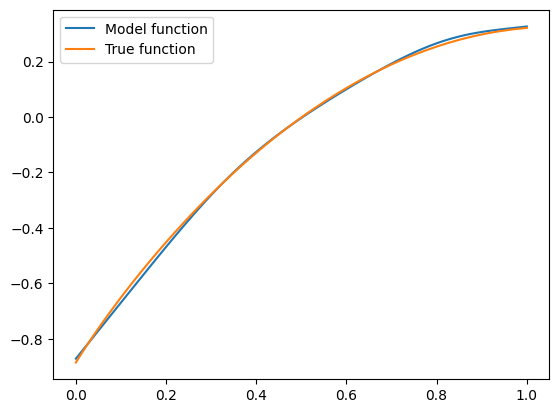
Seems close! Remember, that training and validation sets were generated by taking \(\mathbf{x}\) to be normally distributed with zero mean and standard deviation of 1. So what happens if we feed our model with a vector \(\mathbf{x}\) that is unlikely to be generated by our data distribution? Let’s see what happens for \(\mathbf{x} = (-2, -3, 4)\):

features = torch.tensor([-2., -3., -4.]).repeat(100, 1)
func = partial(model, features)
plt.plot(plot_zs, func(plot_zs).detach().numpy(), label='Model function')
plt.plot(plot_zs, hairy_concave_func(features.numpy(), plot_zs.numpy()), label='True function')

plt.legend()
plt.show()

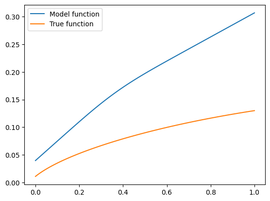
Appears very far away from the true function, but still concave! Even if we feed our model with out-of-distribution data, its predictions may be inaccurate, but they will always satisfy the constraint of concavity. It is built into the model by design. And if this constraint is important for a business application, it’s there!

So now let’s train a fully unconstrained model, with similar MLP layer sizes:

lr = 1e-3
weight_decay = 0.
degree = 20
layer_dims = [4,
              4 * degree,
              3 * degree,
              2 * degree,
              degree]
unconstrained_model, val_loss = train_model(
    train_iter, valid_iter, layer_dims, constrained=False,
    optim_fn=torch.optim.AdamW,
    optim_params=dict(lr=lr, weight_decay=weight_decay))
unconstrained_model = unconstrained_model.cpu()

Note the constrained=False flag we pass to the train_model function. I got a validation loss of \(0.00107\). Doesn’t seem far away from our constrained model. Let’s see what this model, that is not constrained to produce concave functions, has learned. First, let’s try the same “likely” vector \(\mathbf{x}=(-1, 0.1, 0.5)\) as above:

features = torch.cat([
    torch.tensor([-1, 0.1, 0.5]).repeat(100, 1),
    plot_zs.reshape(-1, 1)
], axis=-1)
plt.plot(plot_zs, unconstrained_model(features).detach().numpy(), label='Model function')
plt.plot(plot_zs, hairy_concave_func(features.numpy(), plot_zs.numpy()), label='True function')

plt.legend()
plt.show()

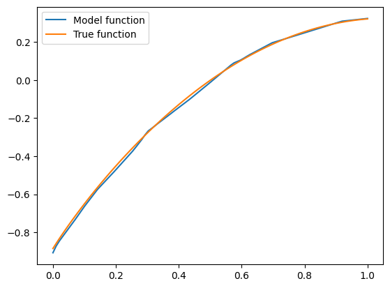
Seems close to the truth, and concave. But is it a coincidence? Let’s try the “unlikely” vector \(\mathbf{x}=(-2, -3, -4)\) we tried above:

features = torch.cat([
    torch.tensor([-2., -3., -4.]).repeat(100, 1),
    plot_zs.reshape(-1, 1)
], axis=-1)
plt.plot(plot_zs, unconstrained_model(features).detach().numpy(), label='Model function')
plt.plot(plot_zs, hairy_concave_func(features.numpy(), plot_zs.numpy()), label='True function')

plt.legend()
plt.show()

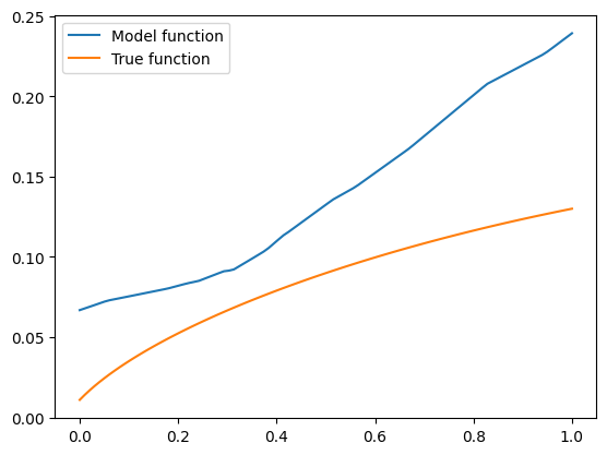
Whoa! The model’s predicted function is both far away from the true function, and not concave! Well, it was expected - after all, a regular MLP model has no mechanism that ensures its predictions are concave.

Summary

In this post we explored an interesting technique to force constraints on the output vectors of neural-network layers, when these constraints are polyhedral cone constraints. We use a library, cddlib, to represent a polyhedral cone using an equivalent “generative” representation, that integrates well with how multi-layer machine learned models are built. This observation allowed us to make sure, by design, that the output of our neural network satisfies the desired property.

In our case, the desired properties were monotonicity, convexity, concavity, or combinations of the above. These are indeed polyhedral cones, and the reason we were interested in them in the first place was constraining continuous functions to have these properties: if the coefficients of a polynomial in the Bernstein basis satisfies these properties, so does the polynomial itself.

The Weyl-Minkowski theorem we used for polyhedral cones is, in fact, more generic. There is a “generative” representation for any set of the form \(\{\mathbf{x} : \mathbf{A} \mathbf{x} \geq \mathbf{b} \}\). In this post we explored only the case of \(\mathbf{b} = \mathbf{0}\). The generator representation for the more general case is a bit more complicated, but not by much. And it also integrates nicely with how PyTorch layers are built. I strongly encourage you to explore it on your own. The cddlib library supports the generic case, so you don’t need to devise the generators yourself. Just understand enough to parse the library’s output.

Finally, as an interesting side note, we now also understand that the last layer of a ReLU network lies in a cone. This is because the ReLU activation before the last layer creates a non-negative vector, and the linear layer that follows contains the generators. The bias only moves the cone to a point that is not the origin. I don’t know of papers that use this interpretation to do something useful, but if you do, please let me know. It sounds interesting.

That’s it! I hope you learned something new about incorporating constraints into neural networks. I certainly have. For me, writing this short series was extremely enlightening. See you soon!

---

1. Frerix, T., Nießner, M., & Cremers, D. (2020). Homogeneous linear inequality constraints for neural network activations. In Proceedings of the IEEE/CVF Conference on Computer Vision and Pattern Recognition Workshops (pp. 748-749). ↩

2. Minkowski, H. (1897). Allgemeine Lehrsätze über die convexen Polyeder. Nachrichten von der Gesellschaft der Wissenschaften zu Göttingen, Mathematisch-Physikalische Klasse, 1897, (pp. 198-220). ↩

3. Weyl, H. (1935). Elementare Theorie der konvexen Polyeder, Comment. Math. Helvetici, 1935, (p7). ↩

4. McMullen, P. (1970). The maximum numbers of faces of a convex polytope. Mathematika, 17(2), 179-184. ↩

5. Avis, D., & Fukuda, K. (1996). Reverse search for enumeration. Discrete applied mathematics, 65(1-3), 21-46. ↩

6. Fukuda, K., & Prodon, A. (1995, July). Double description method revisited. In Franco-Japanese and Franco-Chinese conference on combinatorics and computer science (pp. 91-111). Berlin, Heidelberg: Springer Berlin Heidelberg. ↩