Intro

Occasionally in practice we aim to train models that represent a function of restricted shape, when viewed as a function of one of the features. Formally, we are referring to fitting a function $f(\mathbf{x}, z)$, that is monotone, bounded, convex, or concave in $z$ for every $\mathbf{x}$. The feature $z$ is special in our context - the model $f$ has a special shape as a function of $z$. Here are some examples:

$f(\mathbf{x}, z)$ models insurance premium given features of the policy and the insured person in $\mathbf{x}$, and the coverage in $z$. We would like $f$ to be nondecreasing in $z$ for every $\mathbf{x}$: larger coverage incurs a potentially larger insurance premium.
$f(\mathbf{x}, z)$ models the probability of winning an auction described by features $\mathbf{x}$ and bid $z$. Here, $f$ must be bounded between 0 and 1, since it’s a probability, and nondecreasing in $z$, since higher bids mean potentially chances of winning.
$f(\mathbf{x}, z)$ models utility of an investment of $z$ dollars in a project described by features $\mathbf{x}$. Here it’s reasonable that $f$ is nondecreasing and concave, to model ‘diminishing returns’.

There is a vast amount of literature on learning $f(z)$ with constraints on the shape of $f$ for various families, especially when $f$ is a polynomial. In fact, there’s an entire field of polynomial optimization devoted just to polynomial shape constraints. See this playlist of video lectures, for a great introduction, or just search the web for the term ‘polynomial optimization.’ However, many of the ideas require specialized ‘acrobatics’ that are hard to implement in commodity ML packages we all love: PyTorch and TensorFlow.

There is also the idea of Lattice Networks¹, and a nice TensorFlow library that implements them called TensorFlow Lattice. They are designed for modeling functions of the form $f(\mathbf{x}, \mathbf{z})$, where $\mathbf{z}$ is a vector comprised of several features for which we want to constraint the shape of $f$. They are more generic than the idea I present here, but are also more expensive. This post is about a scalar $z$, meaning that we have only one shape-constrained feature. This lets us do something interesting and specialized for this case.

The idea I present here is probably not new, even though I couldn’t find literature on that. Probably, since I didn’t know what buzzwords to look for. So if you know some prior work I could cite, please let me know!

As customary, the code is available in a notebook you can deploy to Google Colab and play around with. So let’s dive in!

Bernstein polynomials strike again

We already met Bernstein polynomials in our series on polynomial features. So let’s make a short recap of what we learned. Given a degree $n$, we define the polynomials:

\[b_{i,n}(x) = \binom{n}{i} x^i (1-x)^{n-i}.\]

We can see that each $b_{i,d}(x)$ is indeed a polynomial function of $x$ of degree $n$. Moreover, we learned in the series that any polynomial $p(x)$ of degree $n$ can be written as:

\[p(x) = \sum_{i=0}^n a_{i} b_{i,n}(x).\]

In other words, these polynomials are actually a basis for all polynomials of degree $n$. We also learned in this series that this basis is useful for fitting functions on the unit interval $[0, 1]$ with machine learned models without the polynomials going ‘crazy’ and ‘wiggly’ with simple regularization tricks. Finally, we learned that their coefficients give us direct control over the shape of $p(x)$, and in particular:

If $a_0 \leq a_1 \leq \dots \leq a_n$, then $p(x)$ is nondecreasing on $[0, 1]$.
If $a_0 \geq a_1 \geq \dots \geq a_n$, then $p(x)$ is nonincreasing on $[0, 1]$.
If $a_i \in [a, b]$, then $p(x) \in [a, b]$ for any $x \in [0, 1]$.

In other words, nondecreasing or nonincreasing coefficients yield a nondecreasing or nonincreasing polynomial, and imposing a bound on the coefficiens imposes the corresponding bound on the polynomial.

So the basic idea is simple assuming $z \in [0, 1]$. Choose a polynomial degree $n$, feed $\mathbf{x}$ to an arbitrary model that produces the coefficients vector $\mathbf{a} = (a_0, \dots, a_n)$ having the desired monotonicity properties, and let the model’s output be the corresponding polynomial in the Bernstein basis. The basic flow is illustrated below:

increasing_function_model

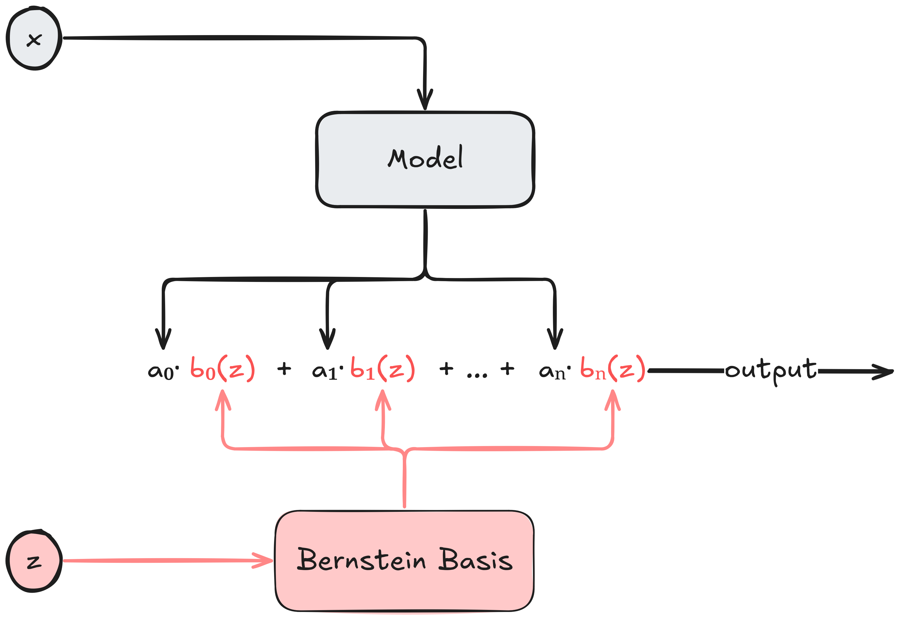
Observe that we don’t really care what the model consuming $\mathbf{x}$ looks like. For all we care, $\mathbf{x}$ can be a free-form text with a description of an insurance policy, and the model consuming $\mathbf{x}$ is our super-duper state-of-the-art transformer that understands insurance policies and produces an embedding vector. But the embedding vector is not arbitrary - it’s a coefficient vector for Bernstein polynomials satisfying a desired shape property. Thus, in this example, the model will have to be fine-tuned for the task of producing the appropriate Bernstein coefficients.

The basic idea of learning a model to predict the coefficient vector of a function is not new. To the best of my knowledge, it dates back to the 1993 paper of Hastie and Tibarshiani², and more papers applying the idea appeared over the years³⁴⁵. That’s why it’s a blog post, rather than a paper. This is one of those posts where I want to understand something by implementing it, and share my understanding and learning experience with the readers.

Before developing the basic idea into a more concrete framework, let’s recall one more interesting fact we learned in the series about Bernstrin polynomials. The Bernstein coefficients control the polynomial locally, in the vicinity of the points on a grid, or a lattice. In this sense, we can think of this basic idea as an enhancement of one-dimensional lattice networks.

Implementing the framework in PyTorch

To implement this idea we need to take care of two details: what happens if $z$ is not in $[0, 1]$, and how do we generate Bernstein coefficients satisfying our desired properties. Then, we shall implement everything in PyTorch.

First, we discuss what happens if $z$ that is not in $[0, 1]$. As mahcine learning practitioners we have a pretty standard set of solutions - feature scaling. For example, if $z$ is assumed to be bounded, we can use simple min-max scaling. For a potentially unbounded, but non-negative feature, such as duration or money, we could scale using $\tanh$, $\arctan$, or an algebraic function such as:

\[\phi_a(z) = \frac{a}{a + z}\]

The choice of the scaling function is where our domain knowledge about $z$ is useful, and this is the “feature engineering” part of our idea. Because feature scaling is typically a part of the data preparation components of a machine learning pipeline, rather than the model, we assume here that our model takes an already scaled $z$.

Now, let’s discuss ensuring that the ‘embedding vector’ $\mathbf{a}$ that our model produces has the right properties (monotonicity / boundedness). This can be achieved by stacking an additional ‘coefficient transform’ layer on top of an existing model. For example, if the last layer of a given model produces a vector $\mathbf{u} = (u_0, \dots, u_n)$, our ‘coefficient transform’ layer produces a nondecreasing $\mathbf{a}$ as using $\mathrm{ReLU}$:

\[a_i = u_0 + \sum_{j=1}^i \mathrm{ReLU}(u_j),\]

or using $\mathrm{SoftPlus}$:

\[a_i = u_0 + \sum_{j=1}^i \mathrm{SoftPlus}(u_j).\]

Below is a $\mathrm{SoftPlus}$ based implementation:

import torch
from torch import nn

class NondecreasingCoefTransform(nn.Module):
    def forward(self, u):
        # We assume that `u` has mini-batch dimensions,
        # and the 'coefficient' dimension is the last one.
        u_head = u[... ,0:1]
        u_tail_relu = nn.functional.softplus(u[..., 1:])
        head_tail = torch.cat([u_head, u_tail_relu], dim=-1)
        return torch.cumsum(head_tail, dim=-1)

Let’s try it out:

u = torch.tensor([-5, 3, -2, 1])
print(NondecreasingCoefTransform()(u))

tensor([-5.0000, -1.9514,  0.1755,  0.4888,  3.5374])

Now we can stack a NondecreasingCoefTransform on top of an existing network, and obtain nondecreasing coefficients.

Now let’s proceed to implementing the idea in PyTorch. First, we need to compute the Bernstein basis using PyTorch using vectorized functions that run well on both CPU and GPU. For simplicity, even though it may not be the ‘best’ way to do it, we shall compute the basis by definition.

It turns out that PyTorch does not have a built-in function to compute the binomial coefficient $\binom{n}{i}$, so let’s implement one. Implementing it directly may cause overflow, since the binomial coefficient is defined in terms of factorials. Moreover, we would like a vectorized implementation that can take many values of $i$ at once. It turns out PyTorch does have the right tools, but in logarithmic space, using the torch.lgamma function that implements the logarithm of the Gamma function. Recall, that the Gamma function generalizes the factorial, since for an integer $n$ we have:

\[\Gamma(n + 1) = n!\]

Therefore,

\[\ln\left(\binom{n}{i}\right) = \ln\left( \frac{n!}{k!(n-k)!} \right) = \ln(\Gamma(n+1)) - \ln(\Gamma(k+1)) - \ln(\Gamma(n - k + 1))\]

So the code for the binomial coefficient in log-space is:

import torch

def log_binom_coef(n: torch.Tensor, k: torch.Tensor):
  return (
      torch.lgamma(n + 1)
      - torch.lgamma(k + 1) 
      - torch.lgamma(n - k + 1)
  )

Let’s see that it works by printing $\binom{5}{i}$ for $i = 0, \dots, 5$:

n = torch.tensor(5)
k = torch.arange(6)
print(log_binom_coef(n, k).exp())

tensor([ 1.,  5., 10., 10.,  5.,  1.])

Appears just right. Now we can implement the Bernstein basis in a naive manner, by definition:

def bernstein_basis(degree: int, z: torch.Tensor):
  """
  Computes a matrix containing the Bernstein basis of a given degree, where
  each row corresponds to an entry in the input tensor `z`.
  """

  # entries of `z` in rows, and basis indices in columns  
  z = z.view(-1, 1) 
  ks = torch.arange(degree + 1, device=z.device).view(1, -1)

  # degree in a tensor to call log_binom_coef
  degree_tensor = torch.as_tensor(degree, device=z.device)

  # now we compute the Bernstein basis by definition
  binom_coef = torch.exp(log_binom_coef(degree_tensor, ks))
  return binom_coef * (z ** ks) * ((1 - z) ** (degree_tensor - ks))

As stated above, this is not the most numerically ‘right’ way work with the Bernstein basis, and it would be more wise to use the well-known De Casteljau’s algorithm, that is both efficient and numerically stable. In fact, in production-quality code that’s what we should do. Maybe even implement a custom CUDA kernel to make it efficient on the GPU. But I chose to avoid adding more complexity by introducing yet another algorithm, and keep this post as straightforward as possible.

So now that we have our ingredients in place, let’s implement a short PyTorch module implementing the idea in the nice diagram we saw above:

from torch import nn

class BernsteinPolynomialModel(nn.Module):
  def __init__(self, x_model, coef_transformer):
    self.coef_model = nn.Sequential([
        x_model,
        coef_transformer
    ])
  
  def forward(self, x, z):
    coefs = self.coef_model(x)
    degree = coefs.shape[-1]
    basis = bernstein_basis(z, degree)
    return torch.sum(coefs * basis, dim=-1)

Coefficient transform components

We already saw a simple transform that takes a vector, and converts it to a vector with non-decreasing components based on the ReLU function. We can do something similar with non-increasing functions using the negative of the ReLU function:

class NonIncreasingCoefTransform(nn.Module):
    def forward(self, u):
        # We assume that `u` has mini-batch dimensions, 
        # and the 'coefficient' dimension is the last one.
        u_head = u[... ,0:1]
        u_tail_relu = -nn.functional.relu(u[..., 1:])
        return torch.cat([u_head, torch.cumsum(u_tail_relu, dim=-1)])

Let’s test it:

print(NonincreasingCoefTransform()(torch.tensor([-5, 3., 2., -1., 3.])))

tensor([ -5.0000,  -8.0486, -10.1755, -10.4888, -13.5374])

Appears to do what we wanted - produces a nonincreasing vector. What if we’re modeling a CDF? Well, then we can add an additional Sigmoid layer on top of a NonDecreasingCoefTransform, that transforms our non-decreasing function whose output are arbitrary numbers, into a non-decreasing function whose output is in $[0, 1]$. Namely, we can use:

nn.Sequential([
	NonDecreasingCoefTransform(),
	nn.Sigmoid()
])

An interesting case is a CDF of a distribution whose support is known to be $[0, 1]$. Then we can model it directly with Bernstein polynomials whose coefficient vector $\mathbf{a}$ satisfies:

\[a_0 = 0 \leq a_1 \leq \dots \leq a_n = 1.\]

To that end, we can use the SoftMax function with a cumulative sum. Assuming that $\mathbf{u} \in \mathbb{R}^n$, we can define:

\[a_i = \frac{\sum_{j=1}^i \exp(u_j)}{\sum_{j=1}^n \exp(u_j)}, \qquad 0 = 1, \dots, n\]

Consequently, the corresponding layer is:

class CDFCoefTransform(nn.Module):
  def forward(self, u):
    zero = torch.zeros_like(u[..., :1])
    cum_softmax = torch.cumsum(nn.functional.softmax(u, dim=-1), dim=-1)
    cdf_coefs = torch.cat([zero, cum_softmax], dim=-1)
    return cdf_coefs

Let’s try it out:

print(CDFCoefTransform()(torch.tensor([-5, 3., 2., -1., 3.])))

tensor([0.0000e+00, 1.4056e-04, 4.1916e-01, 5.7331e-01, 5.8098e-01, 1.0000e+00])

Appears to do what we desire - a non-decreasing vector, going from 0 to 1. Now let’s try to use our components.

Example - learning an increasing function

At first, I wanted to demonstrate it on an application from a domain I know - learning the CDF of auction bids in online advertising. But the data-sets, such as the IPinYou data-set, are too large to handle quickly enough for a blog post. We’ll be using NumPy to implement the synthetic function $f(\mathbf{x}, z)$ we intend to fit, to make plotting and inspection straightforward. When we use it to generate a dataset, we shall transform the NumPy arrays into PyTorch tensors.

import numpy as np

def relu(x):
  return np.maximum(np.zeros_like(x), x)

def softshrink(x, a=0.3):
  return relu(x - a) - relu(-x - a)

def sgn_square(x):
  return x * np.abs(x)

def hairy_increasing_func(x, z):
  x1, x2, x3 = x[..., 0], x[..., 1], x[..., 2]
  return (relu(np.cos(x1 - x2 + x3)) * sgn_square(softshrink(z - np.sin(x1) ** 2))
          + (1 + np.cos(x2 + x3)) * sgn_square(softshrink(z - np.sin(x2) ** 2))
          + (1 + np.cos(x1 - x2)) * sgn_square(softshrink(z - np.sin(x3) ** 2))
          + np.cos(x1 + x2 + x3))

Indeed seems a bit ‘hairy’, so let’s inspect a few examples:

import matplotlib.pyplot as plt

zs = np.linspace(0, 1, 1000)
plt.plot(zs, hairy_increasing_func(np.array([-1, 0.1, 0.5]), zs), label='function 1')
plt.plot(zs, hairy_increasing_func(np.array([1, 0.5, -0.5]), zs), label='function 2')
plt.plot(zs, hairy_increasing_func(np.array([-1.5, 0.8, 0.1]), zs), label='function 3')
plt.legend()
plt.show()

hairy_increasing_functions

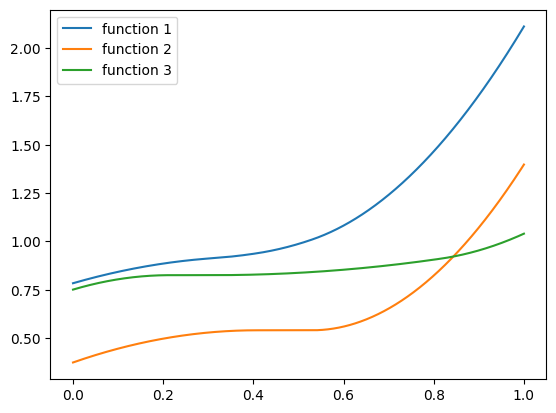
The function uses a few powers of ‘soft-shrink’ that generate ‘flat’ plateaus, to make fitting a bit challenging. The center and slope of these soft-shrink functions are based on trigonometric functions of the component of $\mathbf{x}$. Powers of the soft-shrink function have a discontinuous derivative, and this shall make fitting a bit challenging, even with a small number of features. But it’s possible with polynomials of a high enough degree. As we saw in the polynomial features series - we are not afraid of fitting high-degree polynomial.

Using this function we can generate a PyTorch dataset. The function below generates a data-set of the specified size, and uploads it to the default CUDA GPU if it is available. This is to make our fitting experiments simple and fast when we have a GPU available:

def generate_dataset(n_rows, noise=0.1):
  xs = np.random.randn(n_rows, 3)
  zs = np.random.rand(n_rows)
  labels = hairy_increasing_func(xs, zs) + np.random.randn(n_rows) * noise

  xs = torch.as_tensor(xs).to(dtype=torch.float32)
  zs = torch.as_tensor(zs).to(dtype=torch.float32)
  labels = torch.as_tensor(labels).to(dtype=torch.float32)
  if torch.cuda.is_available():
    xs = xs.cuda()
    zs = zs.cuda()
    labels = labels.cuda()

  return xs, zs, labels

Our next ingredient is a function that builds a PyTorch model. We will be comparing a monotonic model using our BernsteinPolynomialModel class we just implemented, to a regular fully-connected $\mathrm{ReLU}$ network. So here is a function to create a model given layer dimensions that suppotrs both cases:

def make_model(layer_dims, monotone=True):
  # create a fully connected ReLU network
  layers = [
      layer
      for in_dim, out_dim in zip(layer_dims[:-1], layer_dims[1:])
      for layer in [nn.Linear(in_dim, out_dim), nn.ReLU()]
  ]

  if monotone:
    # define a model for x - a ReLU network whose last layer is linear
    x_model = nn.Sequential(*layers[:-1])

    # construct a network for predicting non-decreasing functions
    # the polynomial degree is the output dimension of the last
    # layer.
    return BernsteinPolynomialModel(
        x_model,
        NondecreasingCoefTransform()
    )
  else:
    # define a simple ReLU network - just add a linear layer
    # with one output on top of the ReLU network
    layers.append(nn.Linear(layer_dims[-1], 1))
    return nn.Sequential(*layers)

Let’s verify that even without training, our ‘monotone’ model indeed produces non-decreasing functions of $z$ for each $\mathbf{x}$.

from functools import partial
torch.manual_seed(2024)  # just to make this result reproducible
net = make_model([3, 10, 10, 10])

plot_zs = torch.linspace(0, 1, 100)

func = partial(net, torch.tensor([30., 20, 10]).repeat(100, 1))
plt.plot(plot_zs, func(plot_zs).detach().numpy(), label='Input = [30, 20, 10]')

func = partial(net, torch.tensor([10., 20, 30]).repeat(100, 1))
plt.plot(plot_zs, func(plot_zs).detach().numpy(), label='Input = [10, 20, 30]')

plt.legend()
plt.show()

increasing_random_model

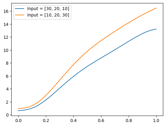
Well, indeed the model appears to generate increasing functions of z.

Now to our last ingredient - model training. Here is a pretty-standard PyTorch training loop, but with a small customization to support monotonic models accepting the features as two parameters $\mathbf{x}, z$, and ‘regular’ models accepting only one features parameter:

from tqdm.auto import tqdm

def train_epoch(data_iter, model, loss_fn, optim, monotone):
  for x, z, label in data_iter:
    if monotone:
      pred = model(x, z)
    else:
      pred = model(torch.cat([x, z.reshape(-1, 1)], dim=-1)).squeeze()
    loss = loss_fn(pred, label)

    optim.zero_grad()
    loss.backward()
    optim.step()

And here is a pretty-standard evaluation loop, doing the same:

@torch.no_grad()
def valid_epoch(data_iter, model, loss_fn, monotone):
  epoch_loss = 0.
  num_samples = 0
  for x, z, label in data_iter:
    if monotone:
      pred = model(x, z)
    else:
      pred = model(torch.cat([x, z.reshape(-1, 1)], dim=-1)).squeeze()
    loss = loss_fn(pred, label)
    epoch_loss += loss * label.size(0)
    num_samples += label.size(0)
  return epoch_loss.cpu().item() / num_samples

Now let’s integrate all ingredients into one function that creates a model and an optimizer, and runs several train+evaluation epochs using the mean squared error loss:

def train_model(train_iter, valid_iter, layer_dims, monotone=True,
                optim_fn=torch.optim.SGD, optim_params=None, num_epochs=100):
  if optim_params is None:
    optim_params = {}

  torch.manual_seed(2024)
  model = make_model(layer_dims, monotone=monotone)
  optim = optim_fn(model.parameters(), **optim_params)
  loss_fn = nn.MSELoss()

  if torch.cuda.is_available():
    model = model.cuda()

  with tqdm(range(num_epochs)) as epoch_range:
    for epoch in epoch_range:
      train_epoch(train_iter, model, loss_fn, optim, monotone)
      epoch_loss = valid_epoch(valid_iter, model, loss_fn, monotone)
      epoch_range.set_description(f'Validation loss = {epoch_loss:.5f}')
  return model, epoch_loss

Now let’s train! First, we create the train and evaluation datasets:

from batch_iter import BatchIter

batch_size = 256
train_iter = BatchIter(*generate_dataset(50000), batch_size=batch_size)
valid_iter = BatchIter(*generate_dataset(10000), batch_size=batch_size)

Now we train a monotonic model. I chose its architecture, the optimizer, and its parameters using hyperparameter tuning with the validation set. But to make this post straightforward, I’m just writing the final hyper-parameters I selected:

lr = 3e-3
weight_decay = 1e-5
degree = 50
layer_dims = [3,
              4 * degree,
              3 * degree,
              2 * degree,
              degree]
model, val_loss = train_model(
    train_iter, valid_iter, layer_dims,
    optim_fn=torch.optim.AdamW,
    optim_params=dict(lr=lr, weight_decay=weight_decay))
model = model.cpu()

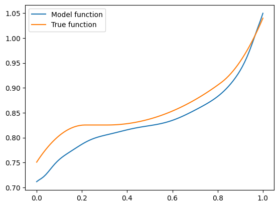
I got a validation loss of 0.0127. Now let’s plot some functions the model learned, and see how they compare to the “true” hairy function we designed. Here is code to produce the function for $\mathbf{x} = (1, 0.5, -0.5)$:

features = torch.tensor([1, 0.5, -0.5]).repeat(100, 1)
func = partial(model, features)
plt.plot(plot_zs, func(plot_zs).detach().numpy(), label='Model function')
plt.plot(plot_zs, hairy_increasing_func(features.numpy(), plot_zs.numpy()), label='True function')

plt.legend()
plt.show()

hairy_bernstein_fit_1

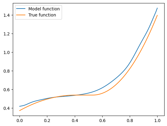
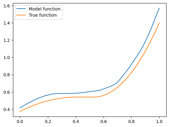
Seems pretty close. Let’s try another one with $\mathbf{x} = (-1.5, 0.8, 0.1)$:

features = torch.tensor([-1.5, 0.8, 0.1]).repeat(100, 1)
func = partial(model, features)
plt.plot(plot_zs, func(plot_zs).detach().numpy(), label='Model function')
plt.plot(plot_zs, hairy_increasing_func(features.numpy(), plot_zs.numpy()), label='True function')

plt.legend()
plt.show()

hairy_bernstein_fit_2

A bit farther away, but not very bad.

Now let’s try training a regular ReLU network on the same dataset and see what functions we have. Its architecture is going to be similar to the $\mathbf{x}$ network from the monotonic example above, but its input dimension is going to be four, instead of three features. This is because now $z$ is not handled separately from the other features. So here is the code to train the network:

lr = 3e-3
weight_decay = 1e-5
degree = 50 # there is no "degree" - it's here just to preserve model architecture.
layer_dims = [4,
              4 * degree,
              3 * degree,
              2 * degree,
              degree]
model, val_loss = train_model(
    train_iter, valid_iter, layer_dims, monotone=False,
    optim_fn=torch.optim.AdamW,
    optim_params=dict(lr=lr, weight_decay=weight_decay))
model = model.cpu()

I got a validation loss of $0.01404$ - slightly worse, but no by much. Let’s see what functions we’re getting for the same two vectors $\mathbf{x}$ we tried before. So here is the code for $\mathbf{x} =(1, 0.5, -0.5)$:

features = torch.cat([
    torch.tensor([1, 0.5, -0.5]).repeat(100, 1),
    plot_zs.reshape(-1, 1)
], axis=-1)
plt.plot(plot_zs, model(features).detach().numpy(), label='Model function')
plt.plot(plot_zs, hairy_increasing_func(features.numpy(), plot_zs.numpy()), label='True function')

plt.legend()
plt.show()

hairy_relu_fit_1

The model function appears monotonic. Is this a coincidence? Well, let’s try our second vector $\mathbf{x} = (-1.5, 0.8, 0.1)$:

features = torch.cat([
    torch.tensor([-1.5, 0.8, 0.1]).repeat(100, 1),
    plot_zs.reshape(-1, 1)
], axis=-1)
plt.plot(plot_zs, model(features).detach().numpy(), label='Model function')
plt.plot(plot_zs, hairy_increasing_func(features.numpy(), plot_zs.numpy()), label='True function')

plt.legend()
plt.show()

hairy_relu_fit_2

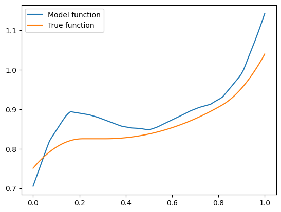
This one isn’t! If we think about it - there is a good reason. Our synthetic dataset was generated by random sampling of standard normal variables - vectors with features are close to zero are more common than those with features farther away. The vector $\mathbf{x} = (1, 0.5, -0.5)$ has components closer to zero than $\mathbf{x} = (-1.5, 0.8, 0.1)$, so there was more training data similar to the former vector than to the latter. Consequently, the model could learn better to represent the functions in the neighbourhood of the former vector. However, when a model is monotone by design, we don’t rely on having enough data for the model to discover monotonic behavior. It’s built into the model.

Summary and discussion

In this post we saw an interesting combination of neural networks with Bernstein polynomials that allow learning shape constraints. This is useful when the shape constraint is actually a constraint, i.e. required for the predictions of the model to be correct from a mathematical or business perspective. Moreover, it’s a form of regularization, since that’s what regularization often is - injecting prior knowledge about the hypothesis class into the fitting procedure.

The idea of constraining coefficients of a function in a given basis to constrain its shape works not only for Bernstein polynomials, but also for the B-Spline basis⁶. Probably also for a variety of other ‘shape-preserving’ bases that I never heard about. So you’re welcome to try this idea with those bases as well, if you believe they suit your needs.

An interesting variation could be designing a polynomial that is monotonic, non-negative, convex or concave over the entire real line $(-\infty, \infty)$. There is an interesting theorem that dates back to Hilbert’s 1888 paper⁷, that any polynomial $p(z)$ of degree $2d$ is non-negative over the entire real line if and only if it is a sum of squares of polynomials. Alternatively, this can be phrased as the existance of a positive-semidefinite matrix $\mathbf{P} \in \mathbb{R}^{d \times d}$ such that the polynomial can be written as

\[p(z;\mathbf{P}) = \begin{pmatrix}1 & z & \dots & z^d\end{pmatrix} \mathbf{P} \begin{pmatrix}1 \\ z \\ \vdots \\ z^d \end{pmatrix}.\]

Any positive semidefinite matrix $\mathbf{P}$ can be decomposed as $\mathbf{P} = \mathbf{V} \mathbf{V}^T$. So just like we predicted the Bernstein coefficient vector $\mathbf{a}$ based on the features $\mathbf{x}$, we could alternatively build a model that learns to predict $\mathbf{V}$.

Since a polynomial is increasing if and only if its derivative is non-negative, we can just take an integral of a non-negative polynomial. Similarly, Convexity can be represented using double-integration of a non-negative polynomial, since a polynomial is convex if and only if its second derivative is non-negative. In boh cases, it’s just multiplying the matrix $\mathbf{P}$ by the corresponding constant representing integration or double integration. Similar “sum of squares” techniques can be used to construct polynomials over an interval, by integrating non-negative polynomials over an interval. See Blekherman et. al. ⁸, Theorem 3.72.

Now let’s get back to the realm of Bernstein polynomials. What happens if we want a polynomial that is both convex and increasing? Or both concave and increasing? This seems useful as well, if we would like to model a utility function that represents diminishing returns. But in this case, we need to impose two constraints on the coefficient vector of the polynomial: one for monotonicity, and another one for concavity. This appears easy with convex optimization solvers that support constraints out of the box, but harder to achieve if we want to train a neural network with PyTorch that produces an coefficient vector that satisfies several constraints. This is exactly what we shall explore in the next post!

You, S., Ding, D., Canini, K., Pfeifer, J., & Gupta, M. (2017). Deep lattice networks and partial monotonic functions. Advances in neural information processing systems, 30. ↩
Hastie, T., & Tibshirani, R. (1993). Varying-coefficient models. Journal of the Royal Statistical Society Series B: Statistical Methodology, 55(4), 757-779. ↩
Ghosal, R., Ghosh, S., Urbanek, J., Schrack, J. A., & Zipunnikov, V. (2023). Shape-constrained estimation in functional regression with Bernstein polynomials. Computational Statistics & Data Analysis, 178, 107614. ↩
Hoover, D. R., Rice, J. A., Wu, C. O., & Yang, L. P. (1998). Nonparametric smoothing estimates of time-varying coefficient models with longitudinal data. Biometrika, 85(4), 809-822. ↩
Huang, J. Z., Wu, C. O., & Zhou, L. (2004). Polynomial spline estimation and inference for varying coefficient models with longitudinal data. Statistica Sinica, 763-788. ↩
Carl De-Boor. A practical guide to splines. (1993) ↩
Hilbert, D. (1888). Über die darstellung definiter formen als summe von formenquadraten. Mathematische Annalen, 32(3), 342-350. ↩
Grigoriy Blekherman, Pablo A. Parrilo, and Rekha R. Thomas. Semidefinite Optimization and Convex Algebraic Geometry. SIAM (2012) ↩