Let the polynomial monster free

Intro

In a recent post by Ben Recht, titled Though Shalt Not Overfit, Ben claims that overfitting in the way that it is colloquially described in data science and machine learning, doesn’t exist. Indeed, there is the famous double descent: trained neural networks that have much more parameters that needed to memorize the training set, tend generalize quite well¹. This includes most of our modern LLMs. So in some cases, models that achieve low training error tend to generalize badly not because their number of parameters is too high, but because it is not high enough!

In his post, Ben Recht claims that what we call “overfitting” is often just a post-hoc rationalization of a model being wrong, and makes us ignore the actual underlying issue that causes it to be wrong. For example, it just may be the case that our model is simply missing some important features. Ben’s post caused some backlash on X with several people disagreeing, such as here, and here where the authors came back to the textbook examples of overfitting high degree polynomials.

In previous posts in this series we saw that high degree polynomials may be very useful in machine learning. We explored the fitting polynomials using the Bernstein basis, and its ability to control the shape of the polynomial that we introduced in in the post “Keeping the polynomial monster under control”. But this time we would like to explore the exact opposite direction - we relinquish control, and set the polynomial monster free. Do high degree polynomials exhibit this double-descent, just like neural networks in general and LLMs in particular? Do they generalize well when the degree is much higher than what is needed to memorize the training data? Are the ML textbooks that show us overfitting with polynomial regression wrong?

Well, apparently they are²³, and this is something we will explore with examples and code in this post in more depth. I first saw it in an X post by @adad8m, who also has plenty of interesting content in her profile for mathematically inclined readers. Surprisingly, even in this simple case of polynomial features in a linear model, the high-degree polynomials we see in textbooks “overfit” simply becaue they are fit incorrectly - using the standard basis. We will explore other polynomial bases, that are available as simple NumPy functions, that memorize the training set and generalize well in absence of any regularization. It turns out there is more to Ben Recht’s post than meets the eye: the way overfitting is taught, as some tradeoff between model complexity and generalization, is nonexistant not only for various neural network families, but also for simple polynomial fitting models! The code for this post is available in a notebook, and you can try it out yourself. Since it’s been a while since I posted about polynomial features, I will attempt to make this post a bit more self contained than previous posts in this series.

Function fitting

Let’s start with a small exercise - of function fitting. Here is a simple function that should be quite challenging for a polynomial to fit:

import numpy as np

def func(x):
    z = np.cos(np.pi * x - 1) + 0.1 * np.cos(2 * np.pi * x + 1)
    return np.cbrt(np.abs(z)) * np.sign(z)

The reason why it is challenging is is due to its shape:

import matplotlib.pyplot as plt

plot_xs = np.linspace(-1, 1, 1000)
plt.plot(plot_xs, func(plot_xs))
plt.show()

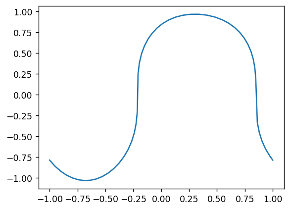
Indeed, its slopes around \(x=-0.25\) and \(x=0.75\) are practically vertical, so any polynomial will have a hard time fitting it. We can now use it to generate noisy training data:

def noisy_func(x, noise=0.1):
    return func(x) + noise * np.random.randn(len(x))

np.random.seed(42)
n = 50
x = 2 * np.random.rand(n) - 1
y = noisy_func(x)

This is what it looks like:

plt.plot(plot_xs, func(plot_xs), label='function')
plt.plot(x, y, 'o', label='data')
plt.legend()
plt.show()

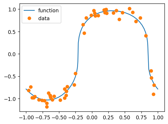
Fitting polynomials

To fit the polynomial to our training data, we use the standard least-squares solved from NumPy:

def fit(degree, feature_matrix_fn):
    # generate polynomial features
    X = feature_matrix_fn(x, degree)
    
    # compute coefficients using the L2 loss
    poly = np.linalg.lstsq(X, y, rcond=-1)[0]
    
    # compute training error (RMSE)
    train_rmse = np.sqrt(np.mean(np.square(X @ poly - y)))
    
    # return coefficients and training error
    return poly, train_rmse

The fit function is a bit generic - it accepts a feature_matrix_fn that transforms each training sample \(x\) into a row vector of polynomials, such as the vector \((1, x, x^2, \dots, x^n)\) for polynomials of degree \(n\), and concatenates these rows in a matrix.

Beyond fitting, we will also need to measure the test error of our fit polynomials, and plot them. To that end, we simply measure the average root mean-squared error between the fit polynomial and the true function at 10,000 points:

def test_fit(degree, feature_matrix_fn, coefs):
    xtest = np.linspace(-1, 1, 10000)
    ytest = feature_matrix_fn(xtest, degree) @ coefs
    test_rmse = np.sqrt(np.mean(np.square(ytest - func(xtest))))
    return xtest, ytest, test_rmse

Now it’s time to discuss why we need this genericity in the form of feature_matrix_fn. It’s a good time to remind ourselves a thing or two about polynomial fitting we learned in this series polynomial features.

Polynomials do not have to be necessarily represented using the standard basis \(\{1, x, x^2, \dots, x^n\}\). For example, consider the polynomial

\[p(x) = 1+2x+3x^2−5x^3 \tag{S}\]

But the same polynomial can also written as \(p(x) = 2−x+2(1.5x^2−0.5)−2(2.5x^3−1.5x). \tag{L}\)

In equation (S) above it’s written in terms of the standard basis and has the coefficients \((1, 2, 3, -5)\), whereas in equation (L) it’s written in terms of the basis \(\{1, x, 1.5x^2-0.5, 2.5x^3-1.5\}\) and has the coefficients \((2, -1, 2, -2)\). This is, by the way, the well-known Legendre polynomial basis, and we shall use it extensively in this post. In general a polynomial can be written as an inner product of two vectors, \(p(x) = \langle \mathbf{P}(x), \mathbf{w} \rangle= \sum_{i=0}^n P_i(x) w_i,\)

where \(\mathbf{P}(x)\) is the vector of basic polynomials, and \(\mathbf{w}\) is the vector of its coefficients. Obviously, \(p(x)\) is a linear function of its coefficients. So when learning a polynomial, the basic polynomials are the features, and the coefficients are the learned parameters of a linear model.

The reason for the genericity in fit is, of course, our desire fit polynomials with different bases \(\mathbf{P}\) to demonstrate a point. For least-squares fitting, the data matrix rows contain the values of the basis functions at each point in the training set. Fortunately, NumPy comes with functions to generate such matrices for a variety of polynomial bases.

Visualizing the fit polynomials

Now let’s try to visually inspect polynomials of various degrees that fit our function. Below is a function that fits a polynomial using a given basis, computes the train and test errors, and plots the fitting results and the polynomial coefficients:

def fit_and_plot(degree, feature_matrix_fn):
    poly, train_rmse = fit(degree, feature_matrix_fn)
    xtest, ytest, test_rmse = test_fit(degree, feature_matrix_fn, poly)
    coef_sum = np.sum(poly)
    fig, axs = plt.subplots(1, 2, figsize=(16, 5))
    fig.suptitle(f'Degree: {degree}, Train RMSE = {train_rmse:.4g}, Test RMSE = {test_rmse:.4g}, Coef Sum = {coef_sum:.4g}')

    axs[0].scatter(x, y)
    axs[0].plot(xtest, ytest, color='royalblue')
    axs[0].plot(xtest, func(xtest), color='red')
    axs[0].set_yscale('asinh')
    axs[0].set_title('Model')

    markerline, stemlines, baseline = axs[1].stem(poly)
    stemlines.set_linewidth(0.5)
    markerline.set_markersize(2)
    axs[1].set_title('Coefficients')
    plt.show()

As expected, it also has the genericity to specify our basis. So let’s try plotting with the standard basis. The feature matrix of the standard basis is constructed using the np.polynomial.polynomial.polyvander function. The “vander” in the name is because the polynomial feature matrix is known as the Vandermonde matrix. Let’s fit a polynomial of degree 1:

fit_and_plot(1, np.polynomial.polynomial.polyvander)

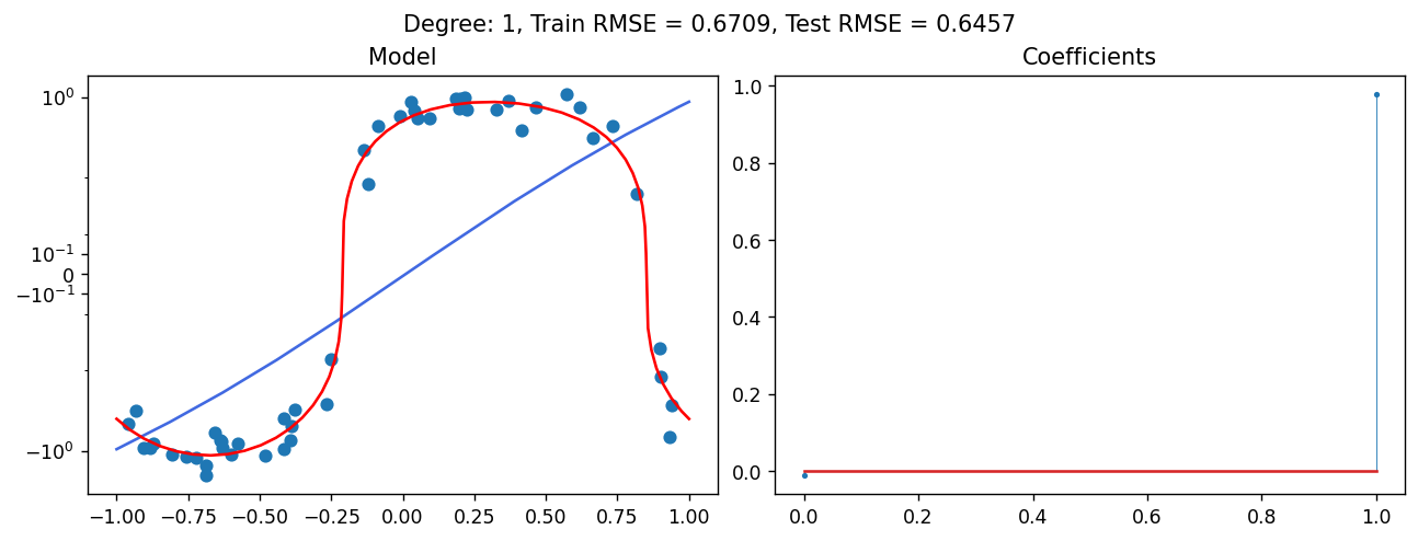
As expected, we got a line, we got a line. The test error is 0.6457. Now let’s try a polynomial of degree 5:

fit_and_plot(5, np.polynomial.polynomial.polyvander)

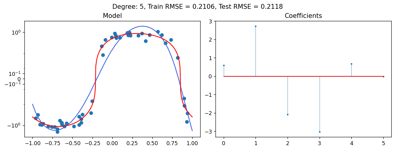
It fits the function better, and the test error is smaller - 0.2118. Now let’s try a polynomial of degree 49. This degree is exactly the “interpolation threshold” - the polynomial degree that can memorize the training set:

fit_and_plot(49, np.polynomial.polynomial.polyvander)

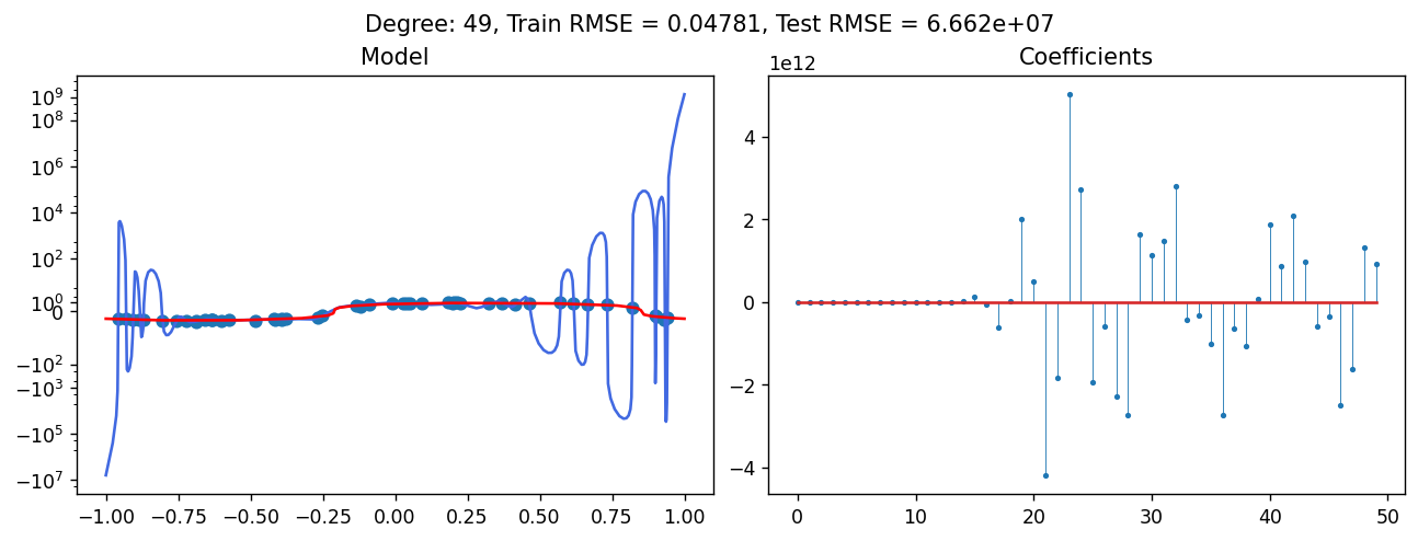
Well, it appears that we’re observing what ML 101 textbooks tell us - we’re overfitting! The polynomial is far away from the function, the train error is almost zero, since we’re exactly fitting the training data up to floating point errors, but the test error is \(\sim 6.7 \times 10^{7}\)! Beyond the interpolation threshold, our polynomial is over-parameterized, meaning it has more parameters than needed to memorize the training set. So what about a polynomial of degree 10,000? Let’s try!

fit_and_plot(10000, np.polynomial.polynomial.polyvander)

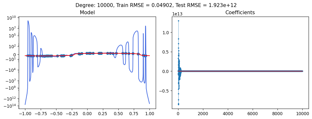
Even worse! But we also observe something suspicious - the coefficients of the high degree polynomial are also large - so is it “overfitting”, or is it something else? Well, let’s try the same exercise with a different basis - the Legendre basis. Its feature matrix is implemented in the np.polynomial.legendre.legvander function. Here is a polynomial of degree 5.

fit_and_plot(5, np.polynomial.legendre.legvander)

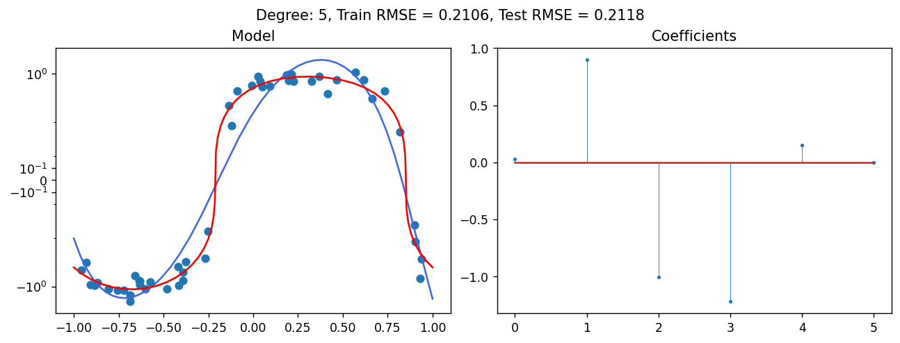
Looks identical to the standard basis. If we think about it - it’s not a surprise. There is a unique least-squares fitting polynomial of degree 5, and it doesn’t matter how we represent it, standard basis, or Legendre basis. Let’s try a degree of 49 - the interpolation threshold:

fit_and_plot(49, np.polynomial.legendre.legvander)

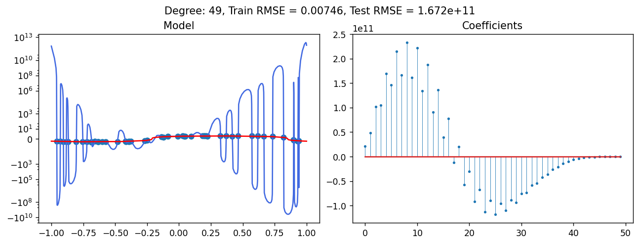
Also looks almost identical to the standard basis. The train error is almost zero. The test error is awful. This is also not a surprise - there is also a unique polynomial of degree 49, the one that exactly passes through the 50 points. So in this case it also doesn’t matter which basis we use. But what happens if we crank up the degree to 10,000? Well, let’s try:

fit_and_plot(10000, np.polynomial.legendre.legvander)

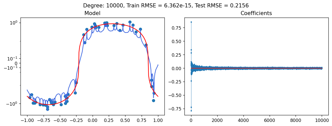
Whoa! That’s interesting! This extremely over-parameterized polynomial both exactly fits the training data points and is pretty close to the true function. The test error is also not bad - \(0.2156\). What happened to our overfitting from ML 101 textbooks? There is no regularization. No control of the degree. But “magically” our high degree polynomial is not that bad! Also look at the coefficients - they are pretty small. We’ll take a deeper look at the coefficients later, but you may notice they appear to follow some trend of decay: coefficients of higher degrees become smaller.

So no it’s time to discuss the two bases. We learned in this series that each basis is coupled with a corresponding “operating region” where it possesses a set of mathematical properties that make it “work well”. I am leaving the meaning of “work well” vague on purpose, but in general it means that it has the right properties to accurately fit functions from a finite amount of training samples in this operating region. For example, in earlier posts we saw that the Bernstein has the interval \([0, 1]\) as its operating region. Moreover, its key property is that its coefficients allow control of the shape of the function. The Legendre basis we just used here has the interval \([-1, 1]\) as its operating region. It turns out to be useful in exactly the opposite scenario - when we do not wish to impose any direct control over its shape. We will try to explain why using intuitive tools later in this post. For the standard basis, the operating region is the complex unit circle. And it’s not a surprise - it’s the foundation of the entire field of Fourier analysis!

It turns out that ML textbooks that use high degree polynomials to demonstrate the balance between “model complexity” and “generalization error” are wrong. The reason is simply the usage of the standard basis. It’s operating reagion is the complex unit circle, it does not possess the mathematical properties required to fit functions of real numbers. The textbooks simply use the wrong tool for polynomial regression, or as Ben Recht pointed in his post, use the wrong features in their linear model!

In this small demo I chose the training and test samples to come from \([-1, 1]\) - this is exactly the operating region of the Legendre basis. In practice, when using high degree polynomial features, you have to first normalize your raw numerical features to the operating region of your basis of choice. You can use standard tools, such as min-max scaling with clipping, or a normalization function such as \(x \to \tanh(\alpha x+ \beta)\). You should never use polynomial features outside the operating region of the basis of your choice!

Error as a function of the degree

Here we saw examples of polynomials of degree 1, 5, 49, and 10,000. But what about the other degrees? Well, let’s plot the test error as a function of the degree and see! Here is a function that plots the train and test errors for a range of polynomial degrees, and also shows the “interpolation threshold” - when the number of parameters equals the number of training poins:

def plot_errors(feature_matrix_fn):
    # define a set of degrees that look nice in a plot - linearly spaced
    # low degrees, and geometrically spaced high degrees.
    degs = np.r_[
        np.sort(np.unique(np.linspace(1, n - 1, 15).astype(int))),
        np.sort(np.unique(np.geomspace(n+1, 100000, 20).astype(int)))
    ]

    # compute train and test errors
    train_errors = np.zeros_like(degs).astype(float)
    test_errors = np.zeros_like(degs).astype(float)
    for i, deg in enumerate(tqdm(degs)):
        poly, train_errors[i] = fit(deg, feature_matrix_fn)
        _, _, test_errors[i] = test_fit(deg, feature_matrix_fn, poly)

    # plot the train and test errors, and the interpolation threshold vertical
    # bar.
    plt.figure(figsize=(16, 6))
    plt.plot(degs, train_errors, label='Train')
    plt.plot(degs, test_errors, label='Test')
    plt.axvline(n - 1, color='royalblue', linewidth=3, linestyle='dotted',
                alpha=0.5)
    plt.axhline(np.min(test_errors), color='olive', linewidth=1, linestyle='dashed',
                alpha=0.5, label=f'Min RMSE = {np.min(test_errors):.3g}')
    plt.ylim([-1e-3, 2 * np.max(test_errors)])
    plt.yscale('asinh', linear_width=1e-3)
    plt.xscale('log')
    plt.xlabel('Degree')
    plt.ylabel('Root Mean Squared Error')
    plt.legend()
    plt.show()

Now let’s plot the errors for the Legendre basis:

plot_errors(np.polynomial.legendre.legvander)

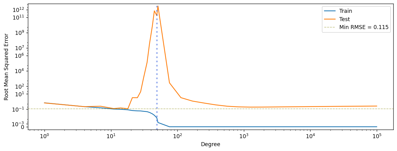
We nicely see the double-descent phenomenon! At the interpolation threshold, the train error drops towards zero, whereas the test error skyrockets. But as the degrees increase, the test error goes down again! What about the standard basis?

plot_errors(np.polynomial.polynomial.polyvander)

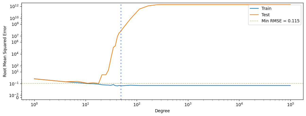
Below the interpolation threshold, the behavior is identical to the Legendre basis below the interpolation threshold. This is because there is only one least-squares fitting polynomial of any degree below 50. But as we cross the interpolation threshold, the train error goes down towards zero, whereas the test error skyrockets. But this is not because of some magical phenomenon called “overfitting” - this is because the standard basis is simply the wrong tool for polynomial fitting.

If we look again at the Legendre polynomial errors plot, we will see that still the low-degree polynomial achieves a better test error than any high-degree polynomial. So why is it interesting that high degree polynomials do not overfit, if the low degree polynomial is better? If you scroll up, you can see that we samples 50 training points. But if we re-run our entire simulation with 600 training points, the plot for the Legendre basis errors is quite different:

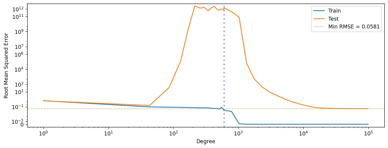
This time, the high degree polynomials generalize even better than any low degree polynomial can. This is similar to what we observe in large neural networks - in the “big data” regime, when we have huge amounts of data, larger models perform better. This is another nail in the coffin of the popular belief that higher model complexity leads to worse generalization! This isn’t true even for polynomial function fitting - the ones that are used to demonstrate “overfitting” in ML textbooks. It’s not about model complexity - it’s about structure!

What makes the standard basis “bad”, and the Legendre basis “good”?

There are mathematically rigorous reasons, pointed out in Schaeffer’s paper on double descent², but here we are aiming for a more intuitive explanation. When fitting with the standard basis, our feature matrix for polynomials of degree \(n\) looks like this:

\[\mathbf{X} = \begin{pmatrix} 1 & x_1 & x_1^2 & \dots & x_1^n \\ 1 & x_2 & x_2^2 & \dots & x_2^n \\ && \vdots & & \\ 1 & x_m & x_m^2 & \dots & x_m^n \\ \end{pmatrix}\]

Intuitively, any two even powers, such as \(x^4\) and \(x^6\), are very similar: both grow quickly as \(x\) gets farther from the origin. The same similarity happens to any two odd powers. This means that the columns of the matrix \(X\) above are highly correlated. As degrees get higher and higher, we’re practically beginning to add almost redundant columns that our linear model has to use as features. Intuitively, a lot of “non-informative” features is what makes the linear model behave badly. This is formally analyzed in Schaeffer’s paper, in the form of the singular values of the matrix \(\mathbf{X}\). In essence, this is also one of the reasons the coefficients of high degree polynomials found using the standard basis were large - such matrices, called ill conditioned matrices, challenge the algorithms used to fit least-squares models.

The Legendre basis is different. Let’s plot the first four polynomials, of degree 0, 1, 2, and 3:

handles = plt.plot(plot_xs, np.polynomial.legendre.legvander(plot_xs, 4))
plt.legend(handles=handles, labels=[f'Degree {i}' for i in range(5)])
plt.show()

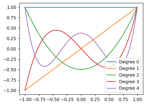
We can see that these polynomials oscilate in \([-1, 1]\)! Higher degrees oscilate more than lower degrees. But not only do they oscilate, but each polynomial oscilates “in different places” than polynomials of lower degrees, meaning it tries to curve up where polynomials of lower degrees curve down, and vice versa. This is formally expressed using the orthogonality property of Legendre polynomials - for any two Legendre basis polynomials, \(P_i(x)\) and \(P_j(x)\) of degrees \(i \neq j\), we have:

\[\langle P_i, P_j \rangle = \int_{-1}^1 P_i(x) P_j(x) dx = 0.\]

Integrals are, of course, just “infinite sums”. Therefore, for enough uniformly sampled points \(x_1, \dots, x_m\), we will have

\[\sum_{k=1}^m P_i(x_k) P_j(x_k) \approx 0\]

Why is it interesting? Well, look at the feature matrix for Legendre polynomials:

\[\mathbf{X} = \begin{pmatrix} P_0(x_1) & P_1(x_1) & \dots & P_n(x_1) \\ P_0(x_2) & P_1(x_2) & \dots & P_n(x_2) \\ & & \vdots & & \\ P_0(x_m) & P_1(x_m) & \dots & P_n(x_m) \\ \end{pmatrix}\]

The orthogonality property means its columns have a little chance to be correlated! Intuitively, it means that adding more and more columns, corresponding to higher and higher degrees, introduces more information the model did not previously had. Fitting a linear model with “informative features”, of course, has a much higher chance of success. But is this informativeness enough? Well, it is not! There are infinitely many polynomials of degree 10,000 that exactly memorize a training set of 50 points. We know there are also bad polynomials of degree 10,000 that memorize the training set - we just found one using the standard basis. And since the Legendre basis is a basis, it can also represent this bad polynomial.

Out of the infinite set of high degree polynomials that exactly memorize the training set, our NumPy least-squares solver chooses only one of them - it chooses the one whose coefficients have the smallest Euclidean norm. The least-squares solver has a “preference” for low-norm coefficients. Exactly this interplay between the way we represent our polynomial and the preference of our optimizer that facilitates this good generalization of high-degree Legendre polynomials.

Let’s try to understand this interplay a bit more. As pointed out above - higher degree Legendre polynomials oscilate more. So we can think of them as a kind of a “frequency domain” - coefficients of higher degrees capture the tendency for more rapid oscilations. The preference for low norm solutions will make the coefficients as small as possible, while still memorizing the training set. That’s why we saw this “decay” of the Legendre polynomial coefficients - the least-squares solver found a polynomial that oscilates as little as possible, while still memorizing the training set. We need the low-degree coefficients to capture the overall shape of the function, but the high degree coefficients, that correspond to rapid oscilations, can be made small, since they only large enough to capture the small deviations from this overall shape.

As evidence, let’s take the polynomial of degree 10,000 we just fit using the Legendre basis, and truncate its degree by using only the first \(k\) basis functions:

def truncated_fit_plots(degree=10000, 
                       truncates=[5, 10, 20, 40],
                       feature_matrix_fn=np.polynomial.legendre.legvander):
    # fit a full degree polynomial, and produce data for plotting
    poly, train_rmse = fit(degree, feature_matrix_fn)

    # data to plot of the full degree polynomial
    xtest = np.linspace(-1, 1, 10000) 
    ytest = feature_matrix_fn(xtest, degree) @ poly

    # create subplots
    n_rows = 2
    n_cols = int(math.ceil(len(truncates) / n_rows))
    fig, axs = plt.subplots(
        n_rows, n_cols, figsize=(n_cols * fig_width, n_rows * fig_height), 
        layout='constrained')
    
    # plot each truncate together with the full degree polynomial
    for trunc_deg, ax in zip(truncates, axs.flatten()):
        trunc_poly = poly[:(trunc_deg + 1)]
        ytest_truncated = feature_matrix_fn(xtest, trunc_deg) @ trunc_poly

        ax.plot(xtest, ytest, color='royalblue', label='full')
        ax.plot(xtest, ytest_truncated, color='red', label=f'truncated')
        ax.set_title(f'Truncate deg={trunc_deg}')
        handles, labels = ax.get_legend_handles_labels()
        
    fig.legend(handles, labels, loc='outside right upper')
    fig.show()
   
truncated_fit_plots()

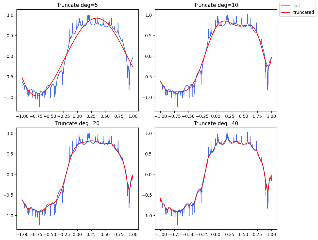
This is a kind of pruning - we are effectively zeroing-out the coefficients of the higher degrees, and using only the lower degree coefficients. We can see that the lowest degrees indeed capture the overall shape, and higher degrees begin to capture the fine deviations from this overall shape towards the noisy dataset. The model actually needs a lot of parameters to be able to learn to differentiate signal from noise!

Deep learning is no different. All optimizers used in practice for deep learning, such as SGD, Adam, or AdamW have some “preference”, just like NumPy’s least-squares solver has a preference for small norm solutions. And just like with our polynomials, it is exactly the interplay between the structure of many deep neural network families and optimizer preference that facilitates this double-descent with neural networks and allows us to scale them to huge sizes without losing generalization power. To the best of my knowledge a good theory has yet to be discovered, but just looking up “overparametrized networks” or “double descent” in your favorite search engine for academic papers will yield tons of literature! Personally, I believe that deeper understanding of this phenomenon with simpler models, such as polynomial fitting, may yield a better theory for deep learning.

But extrapolation! Polynomials don’t extrapolate well!

A common claim is that polynomials “go crazy” if you use them outside of the domain where your training data comes from. Well, let’s try fitting a our function using training data in \([-0.5, 0.5]\), and plotting it together with the fit polynomial in \([-1, 1]\):

np.random.seed(42)
n = 25
x = np.random.rand(n) - 0.5
y = noisy_func(x)

fit_and_plot(10000, np.polynomial.legendre.legvander)

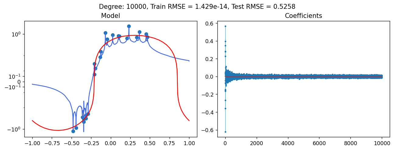
Indeed, we do not have training data beyond \([-0.5, 0.5]\), so we have no way of knowing the true behavior of the function outside of this interval. The best thing we can expect is some “graceful” behavior. Indeed, our super high degree polynomial behaves quite gracefully - it decays towards zero as we get farther away from \([-0.5, 0.5]\). Not bad for extrapolating!

Of course, if we go outside the operating region of the Legendre basis the polynomial will not be graceful at all. It will quickly explode towards infinity. But that’s the whole point - as long as you always normalize your features to the operating region of your polynomial basis - you should expect graceful extrapolation behavior. There is actually no problem “extrapolating” outside of the domain where most of your training data came from, as long as you stay inside the operating region of your basis.

The ML community hasn’t caught up

It turns out that what we saw here has already been discovered a long time ago by the differential equations community. Many natural phenomena are modeled by differential equations, meaning equations whose variable is a function. Oftentimes, the solution cannot be expressed analytically and is approximated.

One popular approximation method is using polynomials, which allow expressing the problem at hand using a set of linear equations in the polynomial coefficients: some of the equations stem from the laws of physics, whereas the others come from (possibly noisy) measurements. The function is then approximated by finding the coefficients stemming from exact fit to the laws of physics, and least-squares fit to the noisy data. Essentially, this is a kind of machine learning.

It turns out thay the differential equations community, and the numerical analysis community in general, already did extensive research on approximating functions using polynomials. It has been known for a very long time that families of orthogonal polynomials “work well”, and this is described extensively in John Boyd’s book⁴. It is unfortunate, but knowledge doesn’t always flow between scientific disciplines, and this is one of those cases. Otherwise, ML textbooks and courses wouldn’t use polynomial regression to demonstrate what is “overfitting”.

Recap

Although polynomials are typically used to demonstrate the need to balance model complexity and generalization, it is a myth. It turns out that the “overfitting” phenomena in this case are just bad numerical behavior of the standard basis, and misunderstanding of the concept of the “operating region” of polynomial bases.

Moreover, typically ML theory deals alot with model classes, also called hypothesis classes. It attempts to answer questions such as: what is is the generalization power of linear regression functions? What about linear classifiers? But it’s not only about model classes. The standard basis of degree 10,000 and the Legendre basis of degree 10,000 represent the same class of models - the class of polynomials of degree 10,000. But we see radically different results with two representations of the same class of models!

The representation, of course, is part of the learning algorithm itself. We can learn our 10,000 degree polynomial in many ways. This is also not a surprise - the same can be said about linear classifiers. A linear classifier can be trained as logistic regression or as a support vector machine - the learning algorithms may have different generalization power, just like two different polynomial bases. This is despite the fact that both yield exactly the same family of models - the family of linear classifiers.

In the next post we shall try to create a scikit-learn component that generates Legendre basis for numerical features, and use it on some real-world datasets. Let’s see what happens when we crank-up the degree on something more serious than just fitting a polynomial curve to noisy samples from a function!

In later posts we shall see how we can use the preference of least-squares solvers towards small norm solutions to facilitate some control, and study another orthogonal polynomial basis - the Chebyshev polynomial basis. You can already take the notebook from this post and try it out yourself - its feature matrix can be constructed using the numpy.polynomial.chebyshev.chebvander function. You will see that it also exhibits double descent. But it’s a bit different, and we shall take a deeper look at the difference between these two bases in the context of machine learning in later posts.

References

1. Belkin, Mikhail, et al. “Reconciling modern machine-learning practice and the classical bias–variance trade-off.” Proceedings of the National Academy of Sciences 116.32 (2019): 15849-15854. ↩

2. Schaeffer, Rylan, Mikail Khona, Zachary Robertson, Akhilan Boopathy, Kateryna Pistunova, Jason W. Rocks, Ila Rani Fiete, and Oluwasanmi Koyejo. “Double descent demystified: Identifying, interpreting & ablating the sources of a deep learning puzzle.” arXiv preprint arXiv:2303.14151 (2023). ↩ ↩²

3. Philipp Benner. “Double descent”. https://github.com/pbenner/double-descent (2022) ↩

4. John P. Boyd. “Chebyshev and Fourier Spectral Methods, 2d. edition”. Dover Publishers (2001). ↩