Behold the power of the spectrum!

Intro

When trying to model a complicated relationship between features, our go-to architectures are typically either neural networks or decision trees. They are well-established, well-studied, and have an abundance of software for training them. So why not?

But sometimes we have some additional requirements. Maybe we want our model to be an increasing / decreasing / convex / concave function of one or more feature. Perhaps we want to measure diminishing returns, and we want it to be both increasing and concave. Or maybe we care about the sensitivity of our model to noise, and want to certify its Lipschitz constant: what happens to the prediction if we slightly change the input?

In the recent interview with Ilya Sutskever there was one interesting insight - perhaps we need neurons to do more compute than they do now. And it immediately rang a bell, and returned me to my Ph.D days - what would be this “more compute” that is useful? Well, maybe a neuron can solve a small optimization problem! So in this post we shall explore an idea that most optimization researchers are familiar with - the eigenvalues of a matrix are solutions to optimization problems. So what can one such neuron do? Turns out quite a lot! This is exactly what we shall explore in this post.

Why eigenvalues? Well, because of a unique combination of three properties. They can model fairly complicated function, we have a lot of theoretical machinery to reason about them, and we can stand on the shoulders of giants and reuse the vast talent and resources invested over decades in their reliable computation.

The notebook for reproducing all the results is here. Feel free to deploy it to Colab and play with it.

Univariate functions

Let’s begin our adventures with a simple case - function of one variable. Suppose we’re given symmetric matrices, \(\mathbf{A}\) and \(\mathbf{B}\), and we define the function:

\[f(x)=\lambda_k(\mathbf{A} + x \mathbf{B}),\]

where \(\lambda_k(\cdot)\) is the \(k\)-th smallest eigenvalue of the given matrix. In general, we will be interested in two things - what kind of functions can we represent, and whether we learn such functions from data.

Our exploration begins with plotting, so let’s implement such a function in a vectorized manner - it will take a vector of inputs, and product a corresponding vector of outputs. Turns out SciPy has excellent tools just for that:

import scipy.linalg as sla
import numpy as np

def univariate_spectral(A, B, k, xs):
  """Computes the vector y[i] = λₖ(A + B * xs[i])."""
  
  # support negative eigenvaue indices,
  #  e.g., k=-1 is the largest eigenvalue
  k = k % A.shape[0]
  
  # create a batch of matrices, one for each entry in xs
  mats = A + B * xs[..., np.newaxis, np.newaxis]
  
  # compute he k-th eigenvalue of each matrix
  return sla.eigvalsh(mats, subset_by_index=(k, k)).squeeze()

Note - we don’t have to pass symmetric matrices. By default, SciPy uses just the entries above the diagonal as if these are the entries of the symmetric matrix. So what do the functions look like? Let’s take two \(3 \times 3\) matrices \(\mathbf{A}\) and \(\mathbf{B}\) and plot the three functions corresponding the three eigenvalues:

import matplotlib.pyplot as plt

def plot_eigenfunctions(A, B, n_rows, n_cols):
  """Plots λₖ(A + B * x) on a grid layout"""
  fig, axs = plt.subplots(n_rows, n_cols, figsize=(3 * n_cols, 2 * n_rows), layout='constrained')
  plot_xs = np.linspace(-5, 5, 1000)
  for k, ax in enumerate(axs.ravel()):
    ax.plot(plot_xs, univariate_spectral(A, B, k, plot_xs))
    ax.set_title(f'$\\lambda_{k}(A + B * x)$')
  plt.show()  


np.random.seed(42)
A = np.random.randn(3, 3)
B = np.random.randn(3, 3)
plot_eigenfunctions(A, B, 1, 3)

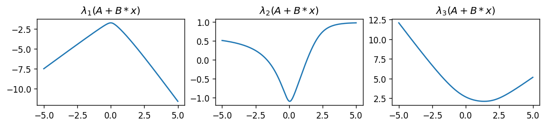
Interesting. The smallest eigenvalue is a concave function, the largest is convex, and the middle appears arbitrary. What happens if we take two \(9 \times 9\) matrices?

np.random.seed(42)
A = np.random.randn(9, 9)
B = np.random.randn(9, 9)
plot_eigenfunctions(A, B, 3, 3)

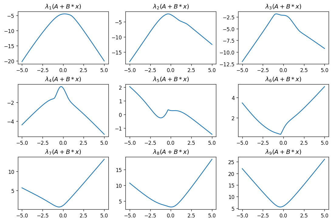
Again, smallest eigenvalue is concave, largest is convex, and the eigenvalues in between are typically neither convex nor concave. Coincidence?

Some of you probably know it is not a coincidence at all. Indeed, recalling elementary results from linear algebra, the smallest eigenvalue of a matrix can be alternatively written as a minimum of quadratic functions:

\[\lambda_1(\mathbf{P}) = \min\{ \mathbf{x}^T \mathbf{P} \mathbf{x} : \| \mathbf{x} \|_2 = 1 \}.\]

These functions may be quadratic in \(\mathbf{x}\), but they are linear in the matrix \(\mathbf{P}\). And a minimum of linear functions is concave. Similarly, the largest eigenvalue is:

\[\lambda_n(\mathbf{P})=\max\{\mathbf{x}^T \mathbf{P} \mathbf{x} : \|\mathbf{x}\|_2=1\},\]

and a maximum of linear functions is convex. So it means our “univariate neuron”, at least for \(\lambda_1\) and \(\lambda_n\), is indeed solving an optimization problem!

But what about the other eigenvalues? There’s a more general version of the above, somewhat less known in the ML community - the Courant-Fischer theorem, for characterizing the \(k\)-th smallest eigenvalue:

\[\lambda_k(\mathbf{P}) = \max_{\mathbf{V} \in \mathbb{R}^{(k-1)\times n}} \min_{\mathbf{x}} \left\{ \mathbf{x}^T \mathbf{P}\mathbf{x} : \| \mathbf{x}\|_2=1,\mathbf{V}\mathbf{x}=\mathbf{0} \right\}.\]

This one appears a bit hairy - so lets dissect it. It can be thought of a game between two players, one chooses \(\mathbf{V}\) and the other one chooses a unit vector \(\mathbf{x}\) that is orthogonal to the rows of \(\mathbf{V}\). The “outer” player aims to maximize their reward, and the “inner” one aims to harm the outer as much as possible.

Consequently, \(\lambda_k\) in general is also solution for an optimization problem. And the farther \(k\) is from the extremities of \(k=1\) and \(k=n\), the “crazier” function it models. If we go back to the plots and look, we can even see that the functions are not necessarily smooth. Indeed, they have “kinks”.

To get a more complete picture, let’s see what happens if we make \(\mathbf{B}\) be not just a symmetric matrix, but a positive-semidefinite one, meaning all its eigenvalues are either positive or zero. It’s easy to make one - just create a random matrix and zero-out all its negative eigenvalues:

def make_psd(B):
  eigvals, eigvecs = sla.eigh(B)
  eigvals_pos = np.maximum(0, eigvals)
  return eigvecs @ np.diag(eigvals_pos) @ eigvecs.T

Now let’s plot!

np.random.seed(42)
A = np.random.randn(9, 9)
B = np.random.randn(9, 9)
plot_eigenfunctions(A, make_psd(B), 3, 3)

That’s interesting - all functions are increasing! What if we take a negative-definite \(\mathbf{B}\)?

np.random.seed(42)
A = np.random.randn(9, 9)
B = np.random.randn(9, 9)
plot_eigenfunctions(A, -make_psd(B), 3, 3)

All are decreasing!

Again, this is not a coincidence. Turns out eigenvalue functions are monotone - if we take a matrix \(\mathbf{A}\) and add the matrix \(x \mathbf{B}\) whose eigenvalues are all non-negative, the entire spectrum of eigenvalues increases. So larger \(x\) results in larger eigenvalues, and vice versa, and we obtain an increasing function. The opposite happens when all eigenvalues of \(\mathbf{B}\) are nonpositive.

Beyond univariate functions

To understand what happens beyond the univariate case, let’s look at functions of two variables given three symmetric matrices \(\mathbf{A}, \mathbf{B}, \mathbf{C}\):

\[f(x, y) = \lambda_k(\mathbf{A} + x\mathbf{B} + y \mathbf{C})\]

For plotting to be convenient, let’s first compute such \(f\) in a vectorized manner:

def bivariate_spectral(A, B, C, k, xs, ys):
  """Computes the vector z[i] = λₖ(A + B * xs[i] + C * ys[i])."""
  
  # support negative eigenvaue indices,
  #  e.g., k=-1 is the largest eigenvalue
  k = k % A.shape[0]
  
  # create a batch of matrices, one for each point (xs[i], ys[i])
  mats = (
      A + B * xs[..., np.newaxis, np.newaxis] 
        + C * ys[..., np.newaxis, np.newaxis]
  )
  
  # compute he k-th eigenvalue of each matrix
  return sla.eigvalsh(mats, subset_by_index=(k, k)).squeeze()

Now we can create surface plots of all eigenvalue functions given the three matrices. Here is the plotting function - nothing special, just a grid of 3D surface plots:

def plot_eigenfunctions_2d(A, B, C, n_rows, n_cols):
  """Plots z = λₖ(A + B * x + C * y) on a grid layout"""
  fig, axs = plt.subplots(
      n_rows, n_cols, figsize=(4 * n_cols, 3 * n_rows),
      subplot_kw={"projection": "3d"}, layout='constrained'
  )
  
  plot_xs = np.linspace(-5, 5, 50)
  grid_xs, grid_ys = np.meshgrid(plot_xs, plot_xs)

  k = A.shape[0]
  for k, ax in enumerate(axs.ravel()[:k]):
    grid_zs = bivariate_spectral(A, B, C, k, grid_xs, grid_ys)
    ax.plot_surface(grid_xs, grid_ys, grid_zs, cmap='viridis')
    ax.set_title(f'$\\lambda_{1 + k}(A + B * x + C * y)$')
  plt.show()  

We’re all set. Let’s plot three eigenvalue functions corresponding to random \(3 \times 3\) matrices:

np.random.seed(42)
A = np.random.randn(3, 3)
B = np.random.randn(3, 3)
C = np.random.randn(3, 3)
plot_eigenfunctions_2d(A, B, C, 1, 3)

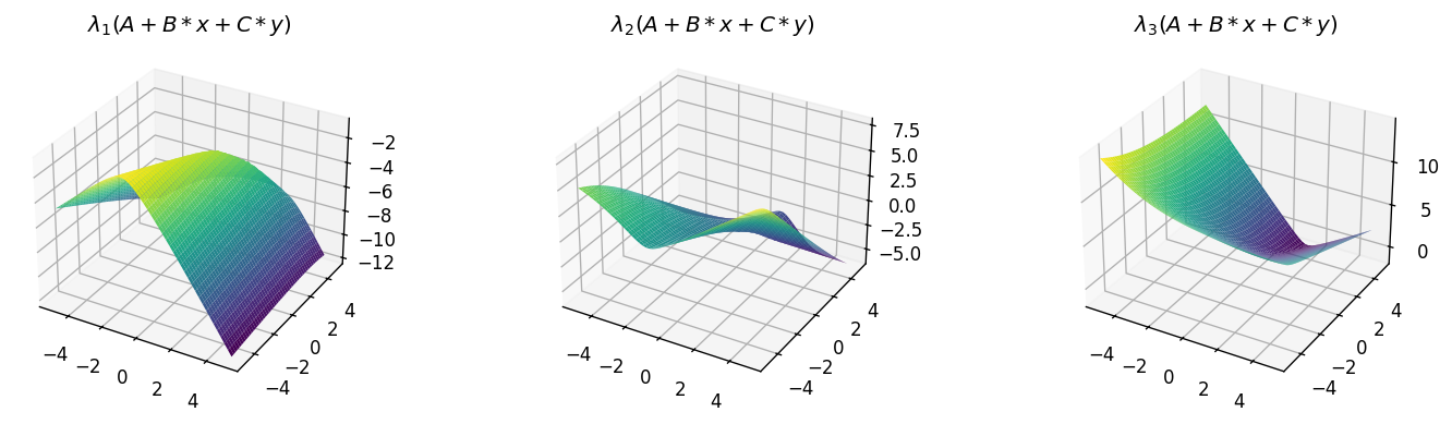
As expected, the smallest eigenvalue produces a concave function, the largest produces a convex one, and the mid eigenvalue produces some arbitrary shape. What if we increase the matrix size to \(9 \times 9\)?

np.random.seed(42)
A = np.random.randn(9, 9)
B = np.random.randn(9, 9)
C = np.random.randn(9, 9)
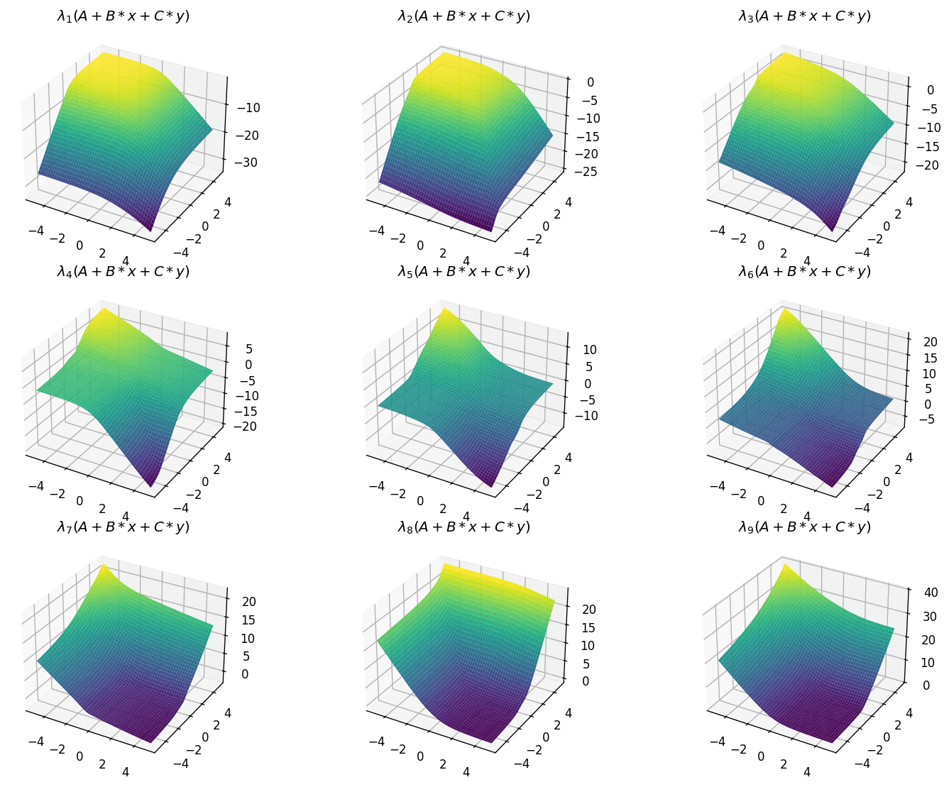
plot_eigenfunctions_2d(A, B, C, 3, 3)

Similar things happen. We can express more “complicated” functions, where the mid eigenvalue \(\lambda_5\) is has the “craziest” shape, whereas the smallest eigenvalue produces a concave function, while the largest yields a convex one.

I assume you can guess what happens when \(\mathbf{B}\) is negative semi-definite, and \(\mathbf{C}\) is positive semi-definite:

np.random.seed(42)
A = np.random.randn(9, 9)
B = np.random.randn(9, 9)
C = np.random.randn(9, 9)
plot_eigenfunctions_2d(A, -make_psd(B), make_psd(C), 3, 3)

As expected, all functions are decreasing in \(x\), and increasing in \(y\). Moreover, the smallest eigenvalue yields a concave function, whereas the largest yields a convex one.

Now why would it be interesting for ML people? Because we can learn the matrices from data! In fact, we can do even more than that - we can predict them. For example, consider a model for predicting the probability of winning a government contract given the contract document and a bid. We use an encoder to transform the document into a symmetric matrix \(\mathbf{A}\) and a positive semi-definite matrix \(\mathbf{B}\), and just compute \(\lambda_k(\mathbf{A} + \mathrm{bid} \cdot \mathbf{B})\), as illustrated below:

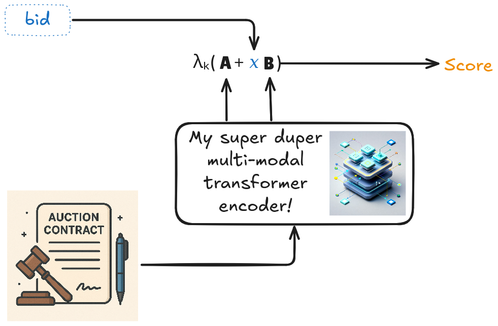
Now we can pass the score to a sigmoid function to obtain a probability that, by design, increases with the bid!

You want a more complex model of two numerical inputs \(x\) and \(y\), but it must increase in \(x\) and decrease in \(y\)? No problem! Just encode your other features into an arbitrary \(\mathbf{A}\), a positive semi-definite \(\mathbf{B}\) , and a negative semi-definite \(\mathbf{C}\), and compute \(\lambda_k(\mathbf{A} + x \mathbf{B} + y \mathbf{C})\).

Training

But can we actually back-propagate through \(\lambda_k\) to learn our encoder? Well, it turns out we can - everything we need is already in PyTorch. In this post, for the sake of the demonstration, we shall do something extremely simple - use a model whose parameters are just \(\mathbf{A}\), \(\mathbf{B}\) and \(\mathbf{C}\) learn them samples of a function of two variables that is concave.

So here is our simple concave function:

def f(x, y):
    return -np.log(np.exp(x-1) + np.exp(y+0.5) + np.exp(-x-y+0.5))

Let’s take a look at its graph and its level sets:

def plot_bivariate(X, Y, Z, show_rmse=False):
    fig = plt.figure(figsize=(10, 5))
    ax = fig.add_subplot(1, 2, 1, projection='3d')
    ax.plot_surface(X, Y, Z)
    ax = fig.add_subplot(1, 2, 2)
    ax.contour(X, Y, Z, levels=20)
    if show_rmse:
        rmse = np.sqrt(np.mean(np.square(Z - f(X, Y))))
        fig.suptitle(f'RMSE = {rmse:.4f}')

x = np.linspace(-3, 3, 300)
y = np.linspace(-3, 3, 300)
X, Y = np.meshgrid(x, y)
plot_bivariate(X, Y, f(X, Y))

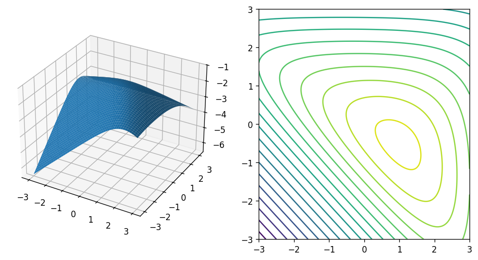
Indeed appears a concave function with some non-trivial shape. The show_rmse flag will be used later when we plot a fitted model and would like to show its approximation error.

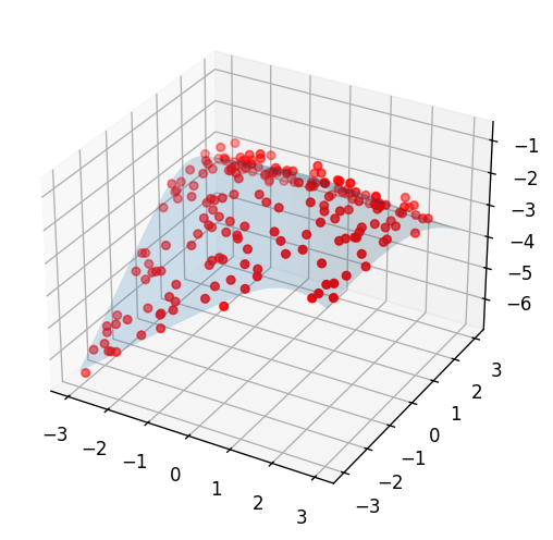
To train a model we shall need two ingredients: training data and a PyTorch module. So let’s generate some training data:

from torch.utils.data import TensorDataset
from torch import as_tensor

def make_trainset(n_train: int = 200, train_noise: float = 0.2):
    np.random.seed(42)
    x = np.random.uniform(-3, 3, n_train)
    y = np.random.uniform(-3, 3, n_train)
    z = f(x, y) + train_noise * np.random.randn(n_train)
    return x, y, z

x_train, y_train, z_train = make_trainset()
ds = TensorDataset(
    as_tensor(x_train), as_tensor(y_train), as_tensor(z_train)
)

Here is what it looks like:

fig = plt.figure(figsize=(5, 5))
ax = fig.add_subplot(1, 1, 1, projection='3d')
ax.scatter(x_train, y_train, z_train, color='red')
ax.plot_surface(X, Y, f(X, Y), alpha=0.2)

Assume that we know we are learning some real-world behavior phenomenon that must be concave. So our PyTorch model shall be the smallest eigenvalue function. This is just a PyTorch re-implementation of the above - it is slightly more generic than we need now to support other eigenvalue indices - not just the smallest. Just like with SciPy, PyTorch also uses just the entries above the diagonal, o we don’t need to worry about symmetry.

import torch
import torch.linalg as tla
from torch import nn

class BivariateSpectral(nn.Module):
    def __init__(self, *, dim: int, eigval_idx: int):
        super().__init__()
        self.eigval_idx = eigval_idx % dim  # modulo - to support negative idx
        self.A = nn.Parameter(torch.randn(dim, dim))
        self.B = nn.Parameter(torch.randn(dim, dim))
        self.C = nn.Parameter(torch.randn(dim, dim))

    def forward(self, x, y):
        # create a batch of matrices, one for each point (x[i], y[i])
        mats = (
            self.A + self.B * x[..., None, None] + self.C * y[..., None, None]
        )

        # compute the eigenvalues
        eigvals = tla.eigvalsh(mats)
        return eigvals[..., self.eigval_idx]

Alright! Let’s train our smallest eigenvalue model! Below is a pretty standard PyTorch training loop:

from torch.utils.data import DataLoader
import math

def train_model(
        model: nn.Module, n_epochs: int = 500, batch_size = 5, lr=1e-3
    ):
    print_every = n_epochs // 10
    dl = DataLoader(ds, batch_size=batch_size, shuffle=True)

    optimizer = torch.optim.Adam(model.parameters(), lr=lr)
    loss_fn = nn.MSELoss()
    for epoch in range(1, 1 + n_epochs):
        epoch_loss = 0.
        for x, y, z in dl:
            optimizer.zero_grad()
            loss = loss_fn(model(x, y), z)
            loss.backward()

            with torch.no_grad():
                epoch_loss += loss.item()
            optimizer.step()

        if epoch == n_epochs or epoch % print_every == 0:
            train_rmse = math.sqrt(epoch_loss / len(ds))
            print(f'Epoch {epoch}, train RMSE: {train_rmse: .4f}')

    return model

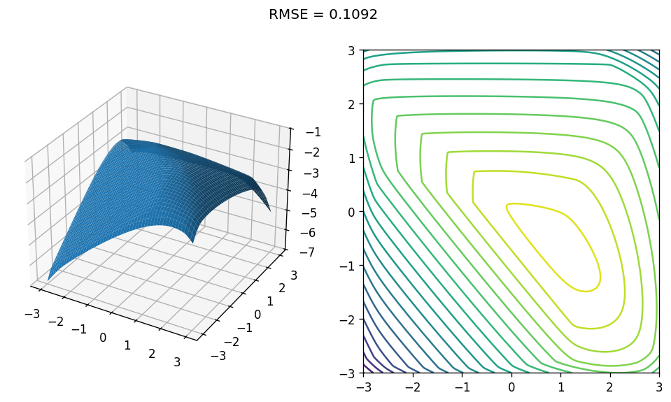
Alright. Let’s try training a concave model with \(3 \times 3\) matrices, and plot it:

model = train_model(BivariateSpectral(dim=3, eigval_idx=0))
with torch.no_grad():
    Z = model(as_tensor(X), as_tensor(Y)).numpy()
plot_bivariate(X, Y, Z, show_rmse=True)

The output:

Epoch 50, train RMSE:  0.0952
Epoch 100, train RMSE:  0.0910
Epoch 150, train RMSE:  0.0884
Epoch 200, train RMSE:  0.0866
Epoch 250, train RMSE:  0.0859
Epoch 300, train RMSE:  0.0862
Epoch 350, train RMSE:  0.0860
Epoch 400, train RMSE:  0.0858
Epoch 450, train RMSE:  0.0858
Epoch 500, train RMSE:  0.0856

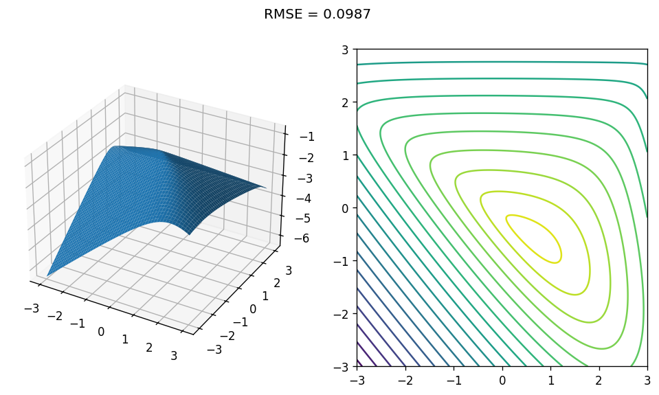
Not bad! Back-propagation appears to be working - the training loss went down, and the plot shows a the model learned something close to the truth.

Now let’s try something interesting - matrices of size \(20 \times 20\). Note, that even one such matrix has more entries than the size of the training set. So such a model is heavily over-parametrized. To make sure we’re converging to the smallest loss I did some tuning, and we need more epochs and a lower learning rate:

model = train_model(
    BivariateSpectral(dim=20, eigval_idx=0), n_epochs=2000, lr=1e-4
)
with torch.no_grad():
    Z = model(as_tensor(X), as_tensor(Y)).numpy()
plot_bivariate(X, Y, Z, show_rmse=True)

Epoch 200, train RMSE:  4.1648
Epoch 400, train RMSE:  2.0389
Epoch 600, train RMSE:  0.5819
Epoch 800, train RMSE:  0.0964
Epoch 1000, train RMSE:  0.0826
Epoch 1200, train RMSE:  0.0811
Epoch 1400, train RMSE:  0.0802
Epoch 1600, train RMSE:  0.0796
Epoch 1800, train RMSE:  0.0793
Epoch 2000, train RMSE:  0.0792

Whoa! This is interesting! Even though the model appears over-parametrized - it does not memorize the training set! Why? Well, one possible explanation is that it is is concave by design, and there appears to be no concave function that can achieve a zero training loss. Also, we see that the model is not “crazy” - its shape also resembles the true one, even if it’s a bit different.

So let’s put our conjecture to a test, and try to fit the mid eigenvalue. This is not a function that is concave by design, and as we saw can have many “crazy” shapes.

model = train_model(
    BivariateSpectral(dim=20, eigval_idx=10), n_epochs=2000, lr=1e-4
)
with torch.no_grad():
    Z = model(as_tensor(X), as_tensor(Y)).numpy()
plot_bivariate(X, Y, Z, show_rmse=True)

Epoch 200, train RMSE:  0.1979
Epoch 400, train RMSE:  0.1031
Epoch 600, train RMSE:  0.0876
Epoch 800, train RMSE:  0.0822
Epoch 1000, train RMSE:  0.0798
Epoch 1200, train RMSE:  0.0786
Epoch 1400, train RMSE:  0.0778
Epoch 1600, train RMSE:  0.0768
Epoch 1800, train RMSE:  0.0764
Epoch 2000, train RMSE:  0.0760

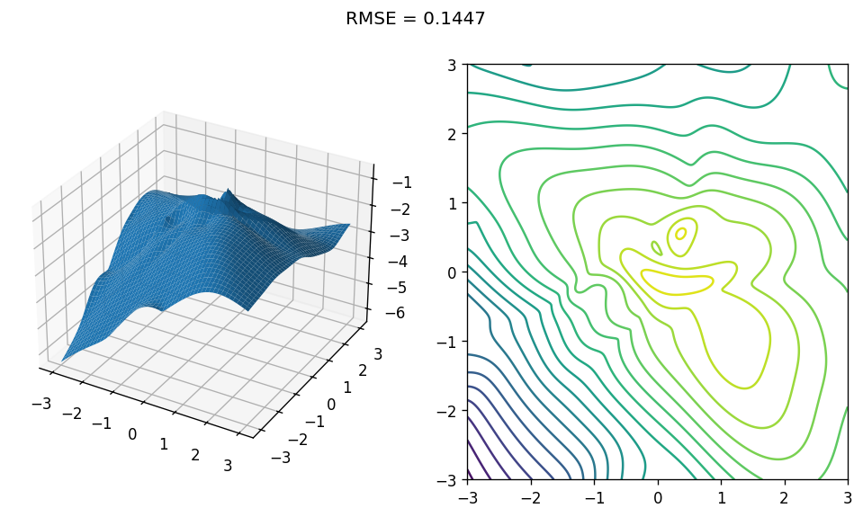
Training error is slightly lower, but apparently does not go down to zero! What happens if we increase the model’s representation power by increasing the size of the matrices? Let’s try the middle eigenvlaue of \(40 \times 40\) matrices:

model = train_model(
    BivariateSpectral(dim=40, eigval_idx=20), n_epochs=2000, lr=1e-4
)
with torch.no_grad():
    Z = model(as_tensor(X), as_tensor(Y)).numpy()
plot_bivariate(X, Y, Z, show_rmse=True)

Epoch 200, train RMSE:  0.1032
Epoch 400, train RMSE:  0.0710
Epoch 600, train RMSE:  0.0668
Epoch 800, train RMSE:  0.0650
Epoch 1000, train RMSE:  0.0639
Epoch 1200, train RMSE:  0.0624
Epoch 1400, train RMSE:  0.0617
Epoch 1600, train RMSE:  0.0609
Epoch 1800, train RMSE:  0.0605
Epoch 2000, train RMSE:  0.0598

Note - training error indeed goes down, so our model gained expressive power. Note - the model has 2460 parameters, much more than our 200 training samples. Yet, the training error does not go to zero, the test error does not explode, and the plot still resembles the true function! So perhaps there is some other property these functions have “by design”, even if we don’t impose shape by using extreme eigenvalues?

Well, there are apparently some interesting properties of these eigenvalue functions worth investigating. So now it would be a good time to do a recap and summarise what we saw, because it appears to be quite a lot to grasp.

Summary

We saw here something that most linear algebra and optimization researchers know for a long time - eigenvalues of symmetric matrices can be used to model functions of various desired shapes. If we know that the real-world phenomenon we aim to learn has some shape, it might be a good idea to model it that way by design. It makes our model sane at inference, because it behaves as we would expect, but it appears to also help train it from data.

Some bibliographic notes. The idea of monotonicity in neural networks was studied before. One prominent line of work is that of deep lattice networks¹ , and mixing monotonicity with convexity and concavity was studied by Runje and Shankaranarayana ². And despite the fact that what I showed here is long known, the idea of just applying the existing knowledge to construct a learnable model from generic eigenvalue functions is, to the best of my knowledge quite recent, and appeared in the 2025 paper by Cook et. al. ³. Their work also proved these models to be universal approximators. Interestingly, universality does not mean the models can exactly memorize a training set of any size, just that they can get arbitrarily close to any function as the model size increases - so it does not contradict our observations here. Moreover, universality is no that important, especially when we care about a specific shape. In fact, in these cases we actually do not want a universal family - we want a family respecting our shape constraints.

Now with this toolbox in mind, we can try to explore other things:

• How do we build a model that learns positve-semidefinite matrices in PyTorch to model increasing / decreasing functions?
• Can we mix and match? For example - build a model that is by design increasing in \(x, z\), decreasing in \(y\), and jointly concave in \((x, y)\)?
• Do we need fully dense matrices? Maybe low-rank / sparse / banded matrices already have enough expressive power?
• What exactly are the properties of eigenvalue functions? What is their representation power? How do eigenvalue functions compare to just plain old ReLU MLPs?
• What are the theoretical interpretations of these eigenvalue functions? Perhaps we can think of them as deep neural networks? Or maybe something else?

In the next posts we shall explore some of these aspects, and maybe more. So stay tuned!

References

---

1. You, Seungil, David Ding, Kevin Canini, Jan Pfeifer, and Maya Gupta. “Deep lattice networks and partial monotonic functions.” Advances in neural information processing systems 30 (2017). ↩

2. Runje, Davor, and Sharath M. Shankaranarayana. “Constrained monotonic neural networks.” In International Conference on Machine Learning, pp. 29338-29353. PMLR, 2023. ↩

3. Cook, Patrick, Danny Jammooa, Morten Hjorth-Jensen, Daniel D. Lee, and Dean Lee. “Parametric matrix models.” Nature Communications 16, no. 1 (2025): 5929. ↩