Paying attention to feature distribution alignment

Intro

Yes, I’m making a joke of the tendency to put the words “attention” and “alignment” in any ML paper 😎. Now let’s see how this provocative title is related to our adventures in the land of polynomial features.

The Legendre polynomial basis serverd us well in recent posts about orthogonality. One interesting thing we saw is that its orthogonality is, in some sense informativeness. Recall, the two polynomials \(P_i\) and \(P_j\) defined on \([-1, 1]\) are orthogonal if

\[\langle P_i, P_j \rangle = \int_{-1}^1 P_i(x) P_j(x) dx = 0,\]

just like two orthogonal vectors - their inner product is zero. The only difference is that the inner product is an integral rather than a sum. But an integral is also an expectation, so if our data points \(x_1, \dots, x_n\) are approximately uniform in \([-1, 1]\), then

\[0 = \int_{-1}^1 P_i(x) P_j(x) dx \sim \frac{2}{n} \sum_{k=1}^n P_i(x_k) P_j(x_k).\]

So any column in the data-set the model observes during training is uncorelated to the other columns coming from the same orthogonal basis, and thus any such column is in some sense informative.

Of course, feature informativeness is not always sufficient but is necessary. And I’d like to devote this post to studying it a bit deeper. Real data isn’t uniformly distributed, and from an intuitive perspective, we can try to “uniformize” it by mapping raw features to quantiles. But does it really work here, both theoretically and practically? This is what we shall explore in this post. The associated notebook for reproducing all results is here.

Weighted orthogonality

Going back to our linear algebra classes, inner products come in many forms. Given a vector of weights \(\mathbf{w} \geq 0\), we can define a weighted inner product:

\[\langle \mathbf{x}, \mathbf{y} \rangle_{\mathbf{w}} = \sum_{i=1}^n x_i y_i w_i.\]

The contribution of every two components at index \(i\) is weighted by the weight \(w_i\).

Similarly, given a weight function \(w(x) \geq 0\) integrable over the domain \(D\). We can define a weighted inner product between two functions on that domain:

\[\langle f, g\rangle_w = \int_{D} f(x)g(x)w(x)dx\]

In particular, we can say that the Legendre basis is orthogonal on \(D = [-1, 1]\) according to the uniform weight \(w(x) = 1\).

Why is it interesting? Well, suppose without loss of generality that \(w(x)\) is normalized such that \(\int_{D} w(x) = 1\). If it’s not, we can always divide it by its integral. So it can be thought of as PDF of some distribution a probability distribution over \(x\). Now the inner product is again just an expectation, and therefore if our data points \(x_1, \dots, x_n\) come from the distribution with PDF \(w\), then:

\[\langle f, g \rangle_w = \mathbb{E}_x \left[ f(x) g(x) \right] \sim \frac{1}{n} \sum_{i=1}^n f(x_i) g(x_i).\]

Given some raw feature \(x\) distributed according to this distribution, the two features \(f(x)\) and \(g(x)\) are uncorrlated. Imagine we know, or can estimate the distribution \(W\) and its PDF \(w\) - how do we come up with a basis of functions orthogonal according to weight of our choice?

The mapping trick

Turns out the differential equations community dealt with similar issues, and came up with many solutions. Here we will consider the simplest one, which I think is best described in a recent survey paper by Shen and Wang¹.

Let’s focus on the Legendre basis that is orthogonal on \([-1, 1]\). Instead of min-max scaling, which we did in previous posts, suppose we use some invertible and differentiable function \(\phi: D \to [-1, 1]\) that maps our feature from its original domain. In terms of the raw feature, our basis functions are

\[Q_i(x) = P_i(\phi(x)).\]

Are they orthogonal? Well, in some sense, they are. Using the change of variable \(y = \phi(x)\), we know from high-school calculus that :

\[0 = \int_{-1}^1 P_i(y) P_j(y) dy = \int_{D} P_i(\phi(x)) P_j(\phi(x)) \phi'(x) dx = \langle Q_i, Q_j \rangle_{\phi'}\]

The conclusion is simple - mapping with \(\phi\) results in orthogonal functions weighted by \(\phi'\). In particular, if \(\phi\) is a CDF of some distribution, then using the basis \(Q_0, Q_1, ...\) will result in uncorrelated features!

So what mapping should we use? If we know or can estimate the CDF \(W\) of our feature, we should use

\[x \to 2W(x) - 1.\]

Indeed, it maps to \([-1, 1]\), and the derivative of this mapping is twice the PDF. Just what we need.

We can, of course, attempt to do mathematical acrobatics to extend this to non-differentiable CDF functions \(W\), but this is not a paper, just a blog post. Finally, we see that this aligns with our intuition at the intro - mapping using a “uniformizing” transformation before computing Legendre polynomials produces an orthogonal basis w.r.t the original raw feature.

A small simulation

We shall sample data from some distributions, and use the above mapping to transform it before computing the Legendre vandermonde matrix. Then, we shall inspect the correlation between columns. Here is a function that accepts a scipy.stats distribution object, and computes the correlation matrix:

import numpy as np

def simulate_correlation(dist, degree=20, n_samples=10000):
    samples = dist.rvs(size=n_samples)
    mapped = 2 * dist.cdf(samples) - 1
    vander = np.polynomial.legendre.legvander(mapped)
    return np.corrcoef(vander.T)

Pretty straightforward - sample, transform, compute Legenre basis functions for each mapped sample, and then correlation between any two resulting features. So let’s try doing some plots. Here is a simulation of our data having the standard Normal distirbution:

import matplotlib.pyplot as plt
import scipy.stats

plt.imshow(simulate_correlation(scipy.stats.norm(0, 1)))
plt.colorbar()
plt.show()

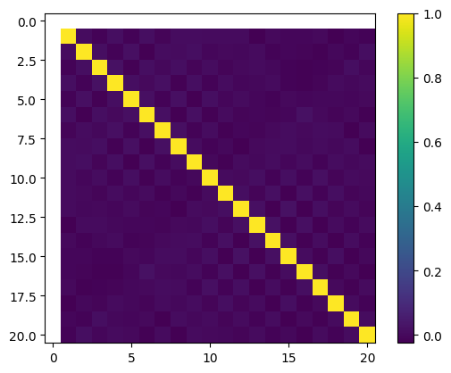
We see a diagonal of ones, and values close to zero outside the diagonal. Well, except for the first row and column - their are the constant function 1, so it has no variance, and thus no covariance. But that’s OK - in models we typically have a separate bias term, and do not include the constant function in our basis.

What about some non-standard normal?

plt.imshow(simulate_correlation(scipy.stats.norm(-5, 10)))
plt.colorbar()
plt.show()

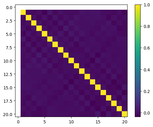
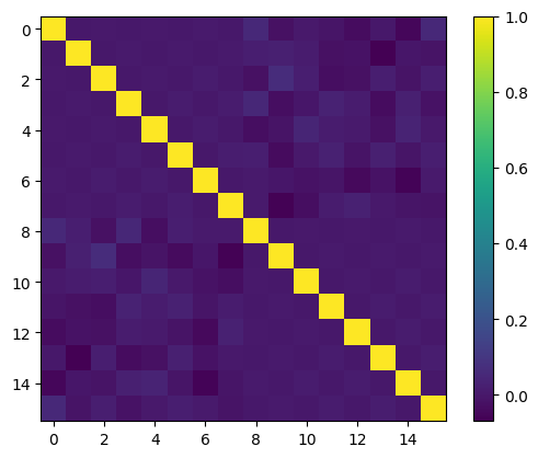
Similar - pairs of features are practically uncorrelated. Their correlation is close to zero. How about some Gamma distribution?

plt.imshow(simulate_correlation(scipy.stats.gamma(8, 2)))
plt.colorbar()
plt.show()

Neat! So if we know our data distribution, we can generate informative non-linear features by composing our CDF-based mapping with the Legendre basis.

What about practice?

In practice we don’t know the data distribution of each column. We can estimate it by various means, such as fitting to some candidate distributions using SciPy. But we can also do another neat approximation - we can use Scikit-Learn’s QuantileTransformer, and it does approximately what we desire. It approximates the CDF, and maps raw features to quantiles using the CDF. We will just have to add one small step to map it from \([0, 1]\) to \([-1, 1]\). Note, that its approximate CDF is non-differentiable - it’s a step function. We haven’t shown anything for a non-differentiable CDF used as a mapping. This is where theory is just a good guide.

Here is a simple pipeline for fitting a linear regression model onto our orthogonal Legendre features, using our previously developed LegendreScalarPolynomialFeatures from the last post. This class doesn’t do anything special - just takes raw feature columns, and computes the Legendre vandermonde matrix.

from sklearn.preprocessing import QuantileTransformer, FunctionTransformer
from sklearn.pipeline import Pipeline

def ortho_features_pipeline(degree=8):
    return Pipeline([
        ('quantile-transformer', QuantileTransformer()),
        ('post-mapper', FunctionTransformer(lambda x: 2*x - 1)),
        ('polyfeats', LegendreScalarPolynomialFeatures(degree=degree)),
    ])

Let’s try applying it to some simulated data and see if we get uncorrelated features. We shall generate two data columns with a Normal and a Gamma distribution, compute features using our pipeline, and plot their correlation matrix:

# two columns - Normal and Gamma
sim_data = np.concatenate([
    scipy.stats.norm(-5, 3).rvs(size=(1000, 1)),
    scipy.stats.gamma(8, 2).rvs(size=(1000, 1)),
], axis=1)

# features
features = ortho_features_pipeline().fit_transform(sim_data)

# plot correlation matrix
coef_mat = np.corrcoef(features.T)
plt.imshow(coef_mat)
plt.colorbar()
plt.show()

Nice! Now let’s try training a linear regression model with our new pipeline.

Testing on real data

Let’s load our beloved california housing dataset and see what we have achieved. Let’s load it, and apply the log transformation we always do to the skewed columns:

import pandas as pd

train_df = pd.read_csv("sample_data/california_housing_train.csv")
test_df = pd.read_csv("sample_data/california_housing_test.csv")

X_train = train_df.drop("median_house_value", axis=1)
y_train = train_df["median_house_value"]

X_test = test_df.drop("median_house_value", axis=1)
y_test = test_df["median_house_value"]

skewed_columns = ['total_rooms', 'total_bedrooms', 'population', 'households']
X_train.loc[:, skewed_columns] = X_train[skewed_columns].apply(np.log)
X_test.loc[:, skewed_columns] = X_test[skewed_columns].apply(np.log)

Now let’s fit a linear regression model and see that it works:

from sklearn.linear_model import LinearRegression
from sklearn.metrics import root_mean_squared_error

pipeline = Pipeline([
    ('ortho-features', ortho_features_pipeline()),
    ('lin-reg', LinearRegression()),
])
pipeline.fit(X_train, y_train)
root_mean_squared_error(y_valid, pipeline.predict(X_valid))

58461.45430931264

Appears to be working. Finally, let’s compare to our min-max scaling strategy we tried in previous posts:

from sklearn.preprocessing import MinMaxScaler

def minmax_legendre_features(degree=8):
    return Pipeline([
        ('scaler', MinMaxScaler(clip=True)),
        ('polyfeats', LegendreScalarPolynomialFeatures(degree=degree)),
    ])

pipeline = Pipeline([
    ('minmax-legendre', minmax_legendre_features()),
    ('lin-reg', LinearRegression()),
])
pipeline.fit(X_train, y_train)
root_mean_squared_error(y_valid, pipeline.predict(X_valid))

60655.269850602985

So at least for the default Legendre polynomial degree, the approximately orthogonal features appear to work quite well. What Let’s try to compare several degrees:

for deg in range(1, 51, 5):
    pipeline = Pipeline([
        ('minmax-legendre', minmax_legendre_features(degree=deg)),
        ('lin-reg', LinearRegression()),
    ])
    pipeline.fit(X_train, y_train)
    minmax_rmse = root_mean_squared_error(y_valid, pipeline.predict(X_valid))

    pipeline = Pipeline([
        ('ortho-features', ortho_features_pipeline(degree=deg)),
        ('lin-reg', LinearRegression()),
    ])
    pipeline.fit(X_train, y_train)
    ortho_rmse = root_mean_squared_error(y_valid, pipeline.predict(X_valid))

    print(f'Degree = {deg}, minmax_rmse = {minmax_rmse:.2f}, ortho_rmse = {ortho_rmse:.2f}')

Degree = 1, minmax_rmse = 64221.56, ortho_rmse = 70346.28
Degree = 6, minmax_rmse = 61380.99, ortho_rmse = 60371.41
Degree = 11, minmax_rmse = 59600.98, ortho_rmse = 58963.64
Degree = 16, minmax_rmse = 59042.73, ortho_rmse = 57859.88
Degree = 21, minmax_rmse = 58242.86, ortho_rmse = 55976.41
Degree = 26, minmax_rmse = 57573.14, ortho_rmse = 55552.21
Degree = 31, minmax_rmse = 57825.45, ortho_rmse = 54469.87
Degree = 36, minmax_rmse = 58483.18, ortho_rmse = 54647.26
Degree = 41, minmax_rmse = 58489.10, ortho_rmse = 55516.40
Degree = 46, minmax_rmse = 58228.28, ortho_rmse = 54655.46

At least on this dataset, the truly orthogonal features appear to be slightly better. What about Ridge regression? Maybe it’s somewhat different?

from sklearn.linear_model import RidgeCV

for deg in range(1, 51, 5):
    pipeline = Pipeline([
        ('minmax-legendre', minmax_legendre_features(degree=deg)),
        ('lin-reg', RidgeCV()),
    ])
    pipeline.fit(X_train, y_train)
    minmax_rmse = root_mean_squared_error(y_valid, pipeline.predict(X_valid))

    pipeline = Pipeline([
        ('ortho-features', ortho_features_pipeline(degree=deg)),
        ('lin-reg', RidgeCV()),
    ])
    pipeline.fit(X_train, y_train)
    ortho_rmse = root_mean_squared_error(y_valid, pipeline.predict(X_valid))

    print(f'Degree = {deg}, minmax_rmse = {minmax_rmse:.2f}, ortho_rmse = {ortho_rmse:.2f}')

Degree = 1, minmax_rmse = 64229.96, ortho_rmse = 70225.96
Degree = 6, minmax_rmse = 61331.81, ortho_rmse = 60228.50
Degree = 11, minmax_rmse = 60766.44, ortho_rmse = 58894.79
Degree = 16, minmax_rmse = 60439.46, ortho_rmse = 57715.60
Degree = 21, minmax_rmse = 60184.00, ortho_rmse = 55896.34
Degree = 26, minmax_rmse = 59718.13, ortho_rmse = 55648.70
Degree = 31, minmax_rmse = 58930.99, ortho_rmse = 54366.58
Degree = 36, minmax_rmse = 58237.94, ortho_rmse = 54820.64
Degree = 41, minmax_rmse = 58440.19, ortho_rmse = 55436.90
Degree = 46, minmax_rmse = 58080.09, ortho_rmse = 54969.96

We see similar results. Our almost orthogonal basis outperforms naive scaling.

Obviously, in practice the degree is a tunable parameter. Its performance should be tested on a validation set, and the best configuraion should then be employed on the test set. But if the same phenomenon happens across many degrees - the conclusion is quite obvious, at least for this dataset.

Summary

This is not a paper, and this is not a thorough benchmark on a variety of data-sets. This is not the point - the point is that even though data speak, theory guides. And its guidance can be oftentimes useful, if you listen carefully.

Now it appears clear why the provocative title fits this post - we indeed paid close attention to the alignment between our non-linear features and the data distribution. This alignment is manifested in the form of the weight of the inner-product space our basis functions live in.

I believe our adventures with continuous numerical feature engineering using polynomials have come to a conclusion. Our next adventures may be about related or totally different subject. It has been a very enlightening experience for me, and I hope it was enlightening for you as well.

References

1. Shen, J. and Wang, L.L., 2009. Some recent advances on spectral methods for unbounded domains. Communications in computational physics, 5(2-4), pp.195-241. ↩