Robustness, interpretability, and scaling of eigenvalue models
This post is part of the series "Eigenvalues as models", and is not self-contained.
Series posts:
-
Behold the power of the spectrum!
- Robustness, interpretability, and scaling of eigenvalue models (this post)
-
I feel the need for Eigen-Speed
-
Interpreting eigenvalue models
-
Cheaper eigenvalue training and inference
-
When Eigenvalues Collide
- Behold the power of the spectrum!
- Robustness, interpretability, and scaling of eigenvalue models (this post)
- I feel the need for Eigen-Speed
- Interpreting eigenvalue models
- Cheaper eigenvalue training and inference
- When Eigenvalues Collide
![]()
Intro
We all want our models to perform well. But some of us would also like our models to be efficient, robust, or interpretable. So in this post we will discuss some mathematical properties of these models that are related to these three pillars. Robustness and interpretability may mean different things to different people, so let’s explain what I mean in this post. As a general note - many things I am going to talk about are true for complex Hermitian matrices, but we focus on real symmetric matrices in the post. So this is the first and the last time I mention complex numbers in this series.
The robustness that we shall explore means robustness to corruption or noise, meaning that bounded changes to the input yield bounded changes to the output, and this bound is known. This is important when we want to know that a small perturbation will not make our model “go wild” and predict something totally unreasonable.
Interpretability can also mean many things. It can be interpretability for us, scientists, so that we can explain what the model does to ourselves. Alternatively, it can mean that we can explain what the model does to a business stakeholder or a regulator. Or in the extreme case, it means we can actually explain to a user why our system made the decision it made based on their input, i.e., why am I not getting a better insurance premium? In this post we shall mostly talk about the first two aspects.
But let’s get started with a small debt I believe I owe you from the previous post - eliminating some of the redundancy.
Eliminating redundancy
We defined our models as
\[f(\mathbf{x}) = \lambda_k \left(\mathbf{A}_0 + \sum_{i=1}^n x_i \mathbf{A}_i \right)\]Some of us may remember from linear algebra that eigenvalues of symmetric matrices are invariant under orthogonal transformations. So the representation of our model is not unique - we can just replace all matrices \(\mathbf{A}_i\) by \(\mathbf{Q}\mathbf{A}_i\mathbf{Q}^\intercal\) for some orthogonal matrix \(\mathbf{Q}\) and obtain exactly the same model. Redundancy, of course, is not unique to this family. Matrix factorization models1 have a similar redundancy. But we can eliminate some of this redundancy.
Since \(\mathbf{A}_0\) is symmetric, it has a spectral decomposition:
\[\mathbf{A}_0 = \mathbf{U} \operatorname{diag}({\boldsymbol\mu}) \mathbf{U}^\intercal,\]where \(\boldsymbol \mu\) is the vector of eigenvalues in some predefined order, such as non-increasing or non-decreasing. Consequently, the model can be written as
\[f(\mathbf{x}) = \lambda_k\left(\operatorname{diag}({\boldsymbol \mu}) + \sum_{i=1}^n x_i (\mathbf{U}^\intercal\mathbf{A}_i \mathbf{U})\right).\]Thus, we can assume that the matrix \(\mathbf{A}_0\) is, for example, diagonal and non-decreasing, without losing any representation power, and assume our model is always of the form:
\[f(\mathbf{x}) = \lambda_k \left( \operatorname{diag}({\boldsymbol \mu}) + \sum_{i=1}^n x_i \mathbf{A}_i \right),\]where \(\boldsymbol \mu\) is a non-decreasing vector, and \(\mathbf{A}_i\) are symmetric matrices. So let’s implement such a model in PyTorch. To that end, we will need a way to represent a non-decreasing vector, which is quite easy - use torch.nn.softplus to generate non-negative gaps, and sum them up. Also, I don’t know what is the right initialization for our \(\boldsymbol \mu\), so I chose uniformly spaced points between -1 and 1:
import torch
from torch import nn

class Nondecreasing(nn.Module):
    def __init__(self, dim: int):
        super().__init__()
        init = torch.linspace(-1, 1, dim)
        self.start = nn.Parameter(init[:1])
        self.increments = nn.Parameter(init.diff().expm1().log())

    def forward(self):
        return torch.cat([
            self.start,
            self.start + nn.functional.softplus(self.increments).cumsum(dim=0)
        ])
Let’s try it out:
Nondecreasing(10)()
tensor([-1.0000, -0.7778, -0.5556, -0.3333, -0.1111,  0.1111,  0.3333,  0.5556,
         0.7778,  1.0000], grad_fn=<CatBackward0>)
Appears to be working. Now, this may not be the best way to parameterize a non-decreasing vector, and you probably can think of other ways, but it appears to works reasonably well when we train models later in this post.
So now we can use it to implement a PyTorch module for the kind of functions we seek. The code is mostly straightforward, and the only thing requires explaining is the initialization of the matrices \(\mathbf{A}_i\), that we shall talk about right after the code snippet:
import torch.linalg as tla

class MultivariateSpectral(nn.Module):
    def __init__(self, *, num_features: int, dim: int, eigval_idx: int):
        super().__init__()
        self.eigval_idx = eigval_idx
        self.mu = Nondecreasing(dim)
        self.A = nn.Parameter(
            torch.randn(num_features, dim, dim) / (math.sqrt(dim) * num_features)
        )

    def forward(self, x):
        # batches of sum of x[i] * A[i]
        nf, dim = self.A.shape[:2]
        feature_mat = (x @ self.A.view(nf, dim * dim)).view(-1, dim, dim)

        # diag(mu) replicated per batch
        bias_mat = torch.diagflat(self.mu()).expand_as(feature_mat)

        # batched eigenvalue computation
        eigvals = tla.eigvalsh(bias_mat + feature_mat)
        return eigvals[..., self.eigval_idx]
Regarding initialization, I am making an educated guess here. It is known2 that the spectrum of \(n \times n\) matrices with random Gaussian entries converges to the semicircle distribution in \([-2\sqrt{n}, 2 \sqrt{n}]\) as \(n\) grows. Moreover, since we will be summing up num_features matrices, it makes sense to initialise our matrices to a normal distribution with a standard deviation of \((\sqrt{n} \cdot \mathtt{num\_features})^{-1}\). Here, too, I don’t know if this is the best initialization, but it works reasonably well.
As a sanity test, let’s try learning the concave function from the previous post:
def f(x, y):
    return -torch.log(torch.exp(x-1) + torch.exp(y+0.5) + torch.exp(-x-y+0.5))

# sample 10000 points on the graph of the function
x = torch.empty(10000).uniform_(-3, 3)
y = torch.empty(10000).uniform_(-3, 3)
xy = torch.stack([x, y], dim=-1)
z = f(x, y) + 0.2 * torch.randn(10000)
Here is a simple training loop to see if the loss decreases - let’s fit a concave model (smallest eigenvalue) with \(5 \times 5\) matrices
import math
from itertools import count

model = MultivariateSpectral(num_features=2, dim=5, eigval_idx=0)
optim = torch.optim.Adam(model.parameters(), lr=1e-3)
batch_size = 10
print_every = 100

cum_loss = 0.
for i, xyb, zb in zip(count(), xy.split(batch_size), z.split(batch_size)):
    loss = (model(xyb) - zb).square().mean()
    cum_loss += loss.detach().item()

    optim.zero_grad()
    loss.backward()
    optim.step()

    if (i + 1) % print_every == 0:
        print(f'Loss = {cum_loss / print_every:.4f}')
        cum_loss = 0.
Loss = 0.4582
Loss = 0.1355
Loss = 0.0774
Loss = 0.0649
Loss = 0.0626
Loss = 0.0520
Loss = 0.0534
Loss = 0.0516
Loss = 0.0464
Loss = 0.0468
OK. The model appears to be learning - the loss is decreasing. So now that we have eliminated most of the redundancy, let’s move on to more interesting stuff.
Spectral stability and its consequences
First, let us recall that any matrix has an associated operator norm - the maximum amount by which it can stretch a unit vector:
\[\|\mathbf{A}\|_{\mathrm{op}} = \max_{\mathbf{x}} \left\{ \|\mathbf{A} \mathbf{x} \|_2 : \|x\|_2 = 1 \right\}\]We have np.linalg.norm and torch.linalg.norm to reliably compute it. Why are we recalling it? Turns out there is a useful consequence of the Weyl’s inequality for symmetric matrices - spectral stability:
So if we take a symmetric matrix \(\mathbf{A}\) and “corrupt” or “perturb” it by another symmetric matrix \(\mathbf{B}\), the resulting eigenvalues do not change by more than \(\|\mathbf{B}\|_{\mathrm{op}}\).
Now, consider our model family, and suppose that the first feature \(x_1\) was perturbed by some noise \(\varepsilon\). By the spectral stability property, our model’s output will not change by more than \(\lvert\varepsilon\rvert \| \mathbf{A}_1 \|_{\mathrm{op}}\). And in general, if our feature vector was perturbed by some noise \(\boldsymbol \varepsilon\), we have:
\[|f(\mathbf{x} + {\boldsymbol \varepsilon}) - f(\mathbf{x})| \leq \Biggl \|\sum_{i=1}^n \varepsilon_i \mathbf{A}_i \Biggr\|_{\mathrm{op}} \leq \sum_{i=1}^n |\varepsilon_i| \| \mathbf{A}_i \|_{\mathrm{op}}\]Now, we have two ways to interpret this bound. First, from the standpoint of robustness - we have a direct bound on the possible change of the prediction as a function of the noise \(\boldsymbol \varepsilon\). For example, if we care about the \(\ell_2\) norm of the noise and want to know what happens when \(\|\boldsymbol \varepsilon\|_2 \leq \alpha\), the Cauchy-Schwarz inequality implies that the model’s prediction changes by at most \(\alpha \sqrt{\sum_{i=1}^n \| \mathbf{A}_i \|^2_{\mathrm{op}}}\).
The second way to think of the bound is from the standpoint of interpretability: one notion of feature importance is a worst-case sensitivity bound. The quantity \(\| \mathbf{A}_i \|_{\mathrm{op}}\) upper-bounds how much the prediction can change when only feature \(x_i\) is perturbed, because a small change of \(\varepsilon\) to feature \(x_i\) will make the model’s prediction change by at most \(\varepsilon \| \mathbf{A}_i \|_{\mathrm{op}}\). So this operator norm is a bound on the effect of feature \(x_i\) on the model’s prediction, just like the magnitude of the coefficients in a linear model.
We can use this knowledge in two ways. First, having trained a model, we can interrogate it for its robustness / feature-importance properties by computing the spectral norms of all feature matrices. Second, we can try to impose a regularization term that imposes a limit on these operator norms. So let’s try the first idea - of observing the operator norms.
Observing stability bounds in practice
We will do it with our beloved California Housing data-set that I use a lot in my blog posts, simply because it’s there on Colab. So let’s load it:
import pandas as pd

train_df = pd.read_csv('sample_data/california_housing_train.csv')
test_df = pd.read_csv('sample_data/california_housing_test.csv')
You may recall from our previous blog posts, that the dataset has four very skewed columns that we typically apply a log transformation to:
import numpy as np

skewed_columns = ['total_rooms', 'total_bedrooms', 'population', 'households']
train_df[skewed_columns] = train_df[skewed_columns].apply(np.log)
test_df[skewed_columns] = test_df[skewed_columns].apply(np.log)
Our final data preprocessing step is plain scaling:
from sklearn.preprocessing import StandardScaler

scaler = StandardScaler().set_output(transform='pandas')
train_scaled = scaler.fit_transform(train_df)
test_scaled = scaler.transform(test_df)

label_scale = scaler.scale_[-1]
We remember the scale of the last column, the label of the data-set, because we want our evaluation metrics in the original units of the label, not in the normalized units. Before training, let’s put our training data in PyTorch tensors - it will be more convenient:
from torch import as_tensor

def to_tensors(df):
    target = 'median_house_value'
    return (
        as_tensor(df.drop(target, axis=1).values),
        as_tensor(df[target].values)
    )

X_train, y_train = to_tensors(train_scaled)
X_test, y_test = to_tensors(test_scaled)

num_features = X_train.shape[1]
n_train = len(X_train)
Alright! So now let’s write our training loop. Here is a fairly standard PyTorch loop for one epoch:
def train_epoch(
        device, net, optimizer, criterion, regularizer, X_batches, y_batches
    ):
    epoch_loss = torch.zeros(1).to(device)
    for x, y in zip(X_batches, y_batches):
        optimizer.zero_grad()
        loss = criterion(net(x), y)
        cost = loss + regularizer(net)
        cost.backward()

        with torch.no_grad():
            epoch_loss += loss * x.shape[0]
        optimizer.step()
    return (epoch_loss / n_train).cpu().item()
The regularizer will become useful later in this post - it’s just an additional penalty beyond the loss. And here is our pretty-standard training loop for the model, but with a twist: we yield intermediate results. Why? It’s convenient to work with - we fully decouple training code from reporting / plotting code:
def train_model_stream(
        net, criterion, *, n_epochs=200, batch_size=10, lr=1e-4, regularizer=None
    ):
    device = 'cuda' if torch.cuda.is_available() else 'cpu'
    regularizer = regularizer or (lambda model: 0.) # by default - no reg.

    net.to(device)
    X_train_batches = X_train.to(device).split(batch_size)
    y_train_batches = y_train.to(device).split(batch_size)
    X_test_device = X_test.to(device)
    y_test_device = y_test.to(device)

    optimizer = torch.optim.AdamW(net.parameters(), lr=lr)
    for epoch in range(1, 1 + n_epochs):
        train_loss = train_epoch(
            device, net, optimizer, criterion, regularizer,
            X_train_batches, y_train_batches
        )

        with torch.no_grad():
            test_loss = criterion(net(X_test_device), y_test_device)
            test_loss = test_loss.cpu().item()

        yield {
            'step': epoch,
            'model': net,
            'train_error': math.sqrt(train_loss) * label_scale,
            'test_error': math.sqrt(test_loss) * label_scale,
        }
This is where we use the label_scale we previously stored - to report the error in the units of the original labels, not the normalized ones. Let’s try a few epochs, to see how it works:
model = MultivariateSpectral(num_features=num_features, dim=5, eigval_idx=2)
criterion = nn.MSELoss()
for event in train_model_stream(model, criterion, n_epochs=5):
    print(event['step'], event['train_error'], event['test_error'], sep='\t')
1	109072.75280327671	99536.88016316161
2	95295.4091119307	89540.08167748511
3	86628.42283455568	82857.71197495822
4	80906.37794419663	78535.01666073261
5	77319.691256485	75821.19027087984
OK - model appears to be training nicely. This trick of yielding lets us do interesting stuff - for example, we can create a new stream that yields train and test errors, together with the spectral norms of the feature matrices:
def add_spectral_norms(stream):
    for event in stream:
        model = event['model']
        with torch.no_grad():
            # remember - we're using only lower-triangular part of each A_i
            matrices_sym = \
                model.A.tril() + model.A.tril(diagonal=-1).transpose(-1, -2)
            norms = tla.matrix_norm(matrices_sym, ord=2)
            norms = norms.ravel().cpu().tolist()

        yield {
            'step': event['step'],
            'train_error': event['train_error'],
            'test_error': event['test_error'],
        } | {
            f'norm_{feature_name}': norm
            for feature_name, norm in zip(feature_names, norms)
        }
Let’s try it out. This time we’ll use the rich library for pretty printing, since the regular Python print doesn’t produce a nice output. So here are 2 training epochs:
from rich.pretty import pprint

model = MultivariateSpectral(num_features=num_features, dim=5, eigval_idx=2)
criterion = nn.MSELoss()
for event in add_spectral_norms(train_model_stream(model, criterion, n_epochs=2)):
    pprint(event)
  {
    'step': 1,
    'train_error': 105523.77536281559,
    'test_error': 97731.75678823328,
    'norm_longitude': 0.12640513479709625,
    'norm_latitude': 0.1759399175643921,
    'norm_housing_median_age': 0.15713410079479218,
    'norm_total_rooms': 0.17977216839790344,
    'norm_total_bedrooms': 0.16544003784656525,
    'norm_population': 0.19817979633808136,
    'norm_households': 0.2670281231403351,
    'norm_median_income': 0.33458226919174194
}
{
    'step': 2,
    'train_error': 94575.6796415192,
    'test_error': 88766.7939206047,
    'norm_longitude': 0.15076042711734772,
    'norm_latitude': 0.1756560057401657,
    'norm_housing_median_age': 0.1784549206495285,
    'norm_total_rooms': 0.18125228583812714,
    'norm_total_bedrooms': 0.15172506868839264,
    'norm_population': 0.19934602081775665,
    'norm_households': 0.26696428656578064,
    'norm_median_income': 0.47850197553634644
}
Nice! So now we can iterate and do live-plotting of everything! This is a lengthy function with mostly boilerplate that plots two graphs - one with train/test errors, and another one with spectral norms of feature matrices. I added comments to make the code clear, but the principle is simple: we create empty plots, and gradually update them as new events arrive.
import matplotlib.pyplot as plt

def plot_progress(events, max_step):
    # create a plot with two axes - one for errors, one for norms
    fig, (err_ax, norm_ax) = plt.subplots(
        2, 1, figsize=(8, 8), layout='constrained'
    )

    # create empty line objects
    def plot_empty(ax, label):
        return ax.plot([], [], label=label)[0]

    line_dict = {
        'train_error': plot_empty(err_ax, 'train error'),
        'test_error': plot_empty(err_ax, 'test error'),
    } | {
        f'norm_{feature_name}': plot_empty(norm_ax, feature_name)
        for feature_name in feature_names
    }

    # setup axis properties
    err_ax.set_title("Error")
    norm_ax.set_title("Matrix norms")
    for ax in (err_ax, norm_ax):
        ax.set_xlabel("Step")
        ax.set_xlim(0, max_step)
        ax.grid(True)
        ax.legend()


    # display figure and obtain its handle
    h = display(fig, display_id=True)
    plt.close(fig)

    # iterate over events and update the plot
    min_test_error = float('inf')
    for event in events:
        step = event['step']
        min_test_error = min(min_test_error, event['test_error'])
        err_ax.set_title(f'Error (min test err = {min_test_error:.2f})')

        for key, line in line_dict.items():
            value = event[key]
            x, y = line.get_data(orig=True)
            line.set_data(np.append(x, step), np.append(y, value))

        for axs in (err_ax, norm_ax):
            axs.relim()
            axs.autoscale_view()

        fig.canvas.draw()
        h.update(fig)
Alright! Let’s use it to train a mid-eigenvalue model with \(5 \times 5\) matrices:
def live_plot_training(dim, n_epochs):
model = MultivariateSpectral(
num_features=num_features, dim=dim, eigval_idx=dim // 2
)
criterion = nn.MSELoss()
events = add_spectral_norms(train_model_stream(
model, criterion, n_epochs=n_epochs
))
plot_progress(events, max_step=n_epochs)
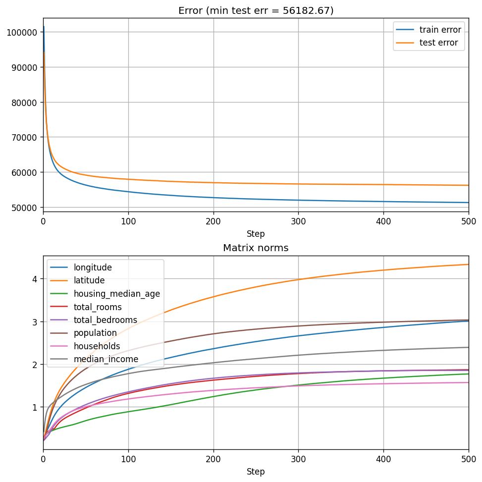
live_plot_training(5, 500)

OK. We can see that the model is learning, and after 500 epochs we observe that the resulting model’s strongest three features are longitude, latitude, and population. What happens when we increase model size? Let’s try \(15 \times 15\) matrices:
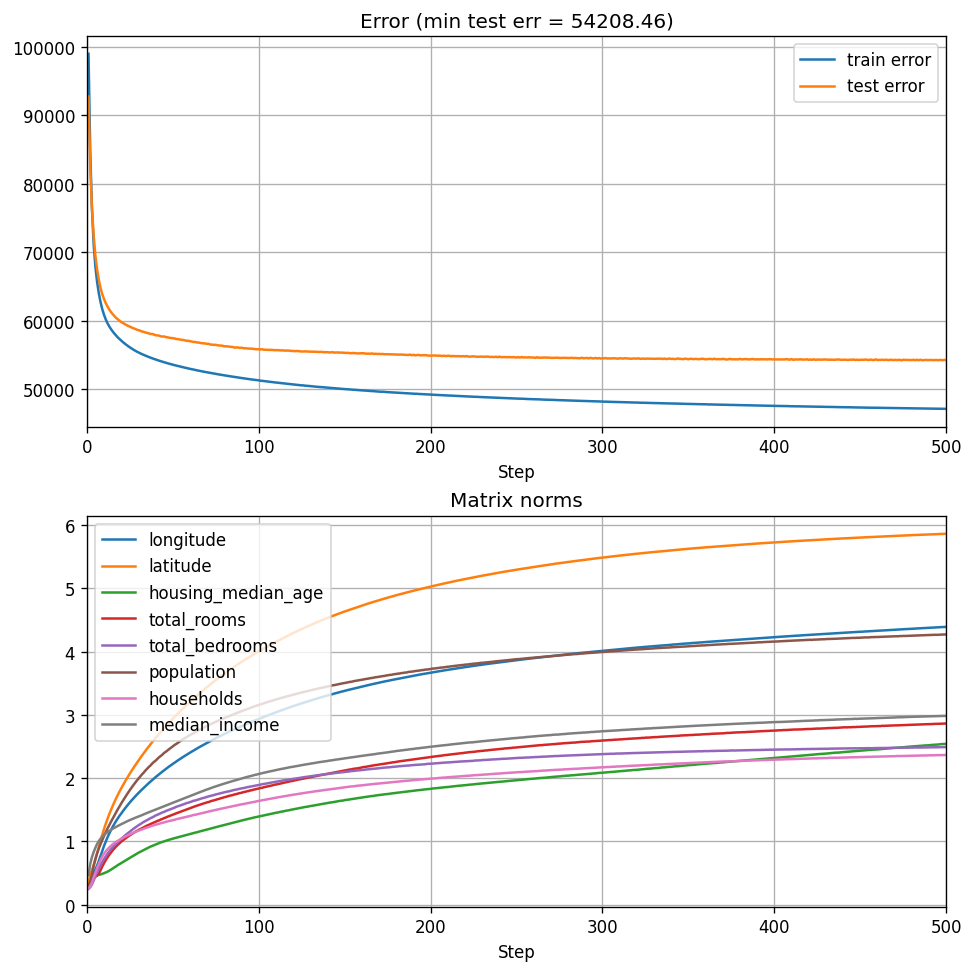
live_plot_training(15, 500)
We see that the test loss decreases with the model size, and even though the ranking between features is slightly different, the three strongest features remain longitude, latitude, and population. But we also see something else - the matrix norms continue growing. Apparently, after 500 epochs, the model’s parameters do not appear to be converging. Perhaps a more thorough hyper-parameter tuning would help, I don’t know. But I chose a conservative option of a small learning rate and many epochs for a reason - to show that scaling model size improves performance, while keeping our model’s ability to be interpretable almost as if it was linear.
Let’s go even further up, to \(30 \times 30\) matrices:
live_plot_training(30, 500)
We see that the train and test errors go further down, and the three features previously at the top remain there. Again - scaling up improves performance, while keeping interpretability and computable robustness bounds.
So what we got here is really interesting! We have a model that is nonlinear and improves with scaling, while remaining interpretable in terms of feature sensitivity / importance, and we have an easy way to compute global sensitivity bounds (which can be loose).
As a reference, if you try fitting a gradient-boosted decision forest using XGBoost, you’ll observe a test error of approximately $48,000. So the eigenvalue model we see here isn’t close to what trees can achieve, but tree ensembles are often discontinuous and don’t come with simple global sensitivity/Lipschitz certificates in the same way. So it’s a tradeoff.
Sensitivity control
Another way we can use our understanding of the stability properties is to regularize the model by either imposing a bound on the maximum spectral norm, or adding a regularization term that penalizes the spectral norms, so our training code will be minimizing
\[\min_{\mathbf{A}_{1:n}, \boldsymbol\mu} \quad \underbrace{\frac{1}{N} \sum_{i=1}^N (f(\mathbf{x}_i;\mathbf{A}_{1:n}, {\boldsymbol \mu}) - y_i)^2}_{\mathrm{loss}} + \underbrace{\alpha \sum_{i=1}^n \| \mathbf{A}_i \|_{\mathrm{op}}}_{\mathrm{penalty}}\]This is where we shall use the regularizer parameter of our training function that I promised you:
def live_plot_reg_training(dim, n_epochs, reg_coef):
    model = MultivariateSpectral(
        num_features=num_features, dim=dim, eigval_idx=dim // 2
    )

    def penalty(net):
        matrices_sym = \
            net.A.tril() + net.A.tril(diagonal=-1).transpose(-1, -2)
        norms = tla.matrix_norm(matrices_sym, ord=2)
        return reg_coef * norms.sum()

    criterion = nn.MSELoss()
    events = add_spectral_norms(train_model_stream(
        model, criterion, n_epochs=n_epochs, regularizer=penalty
    ))
    plot_progress(events, max_step=n_epochs)
Let’s try it out with \(15 \times 15\) matrices:
live_plot_reg_training(15, 500, 1e-3)
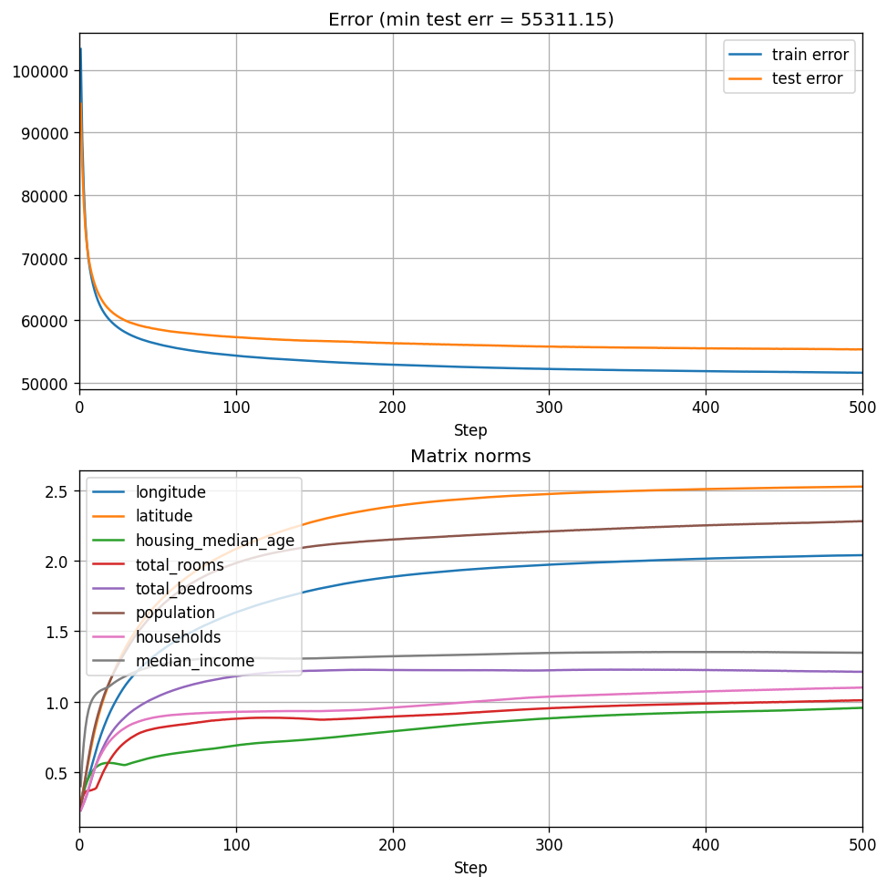
We can see that the spectral norms are smaller than our previous attempt with \(15 \times 15\) matrices above, norm growth appears to stabilize, but performance appears similar. Just the gap between the top four features and the rest of the features became more pronounced - that’s the effect of delicate regularization. A larger regularization coefficient may even drive some of the matrices towards zero, similarly to \(\ell_1\) regularization in Lasso.
Imposing such a regularizer with standard PyTorch optimizers, rather than a dedicated optimizer, may not be the optimal (pun intended!) thing to do, and some of you can probably think of better ways. But that’s beside the point - the point is that we can, in principle, regularize the spectral norm to control the model’s sensitivity to feature perturbations. And that is quite powerful.
So now after we’ve seen plenty of stuff - it’s time for a recap.
Summary
We saw that matrix eigenvalues let us find a nice sweet-spot between several opposing forces - performance, robustness, and interpretability. Beyond just models for tabular data, this nice idea can also be employed for another use case we haven’t yet discussed - ensembling. There, too, we care about the ensemble’s prediction to behave “sensibly” w.r.t the predictions of the individual models, and there too we may care about robustness and interpretability. So it’s nice to have a learnable ensembling technique that both improves with scaling, but remains robust and somewhat interpretable.
We will study other mathematical properties in future posts that will let us understand on a deeper level what kind of information we can elicit from those models, but as of now we have a slightly more urgent concern: training is slow. We need many epochs, and each epoch is expensive. This makes experimentation hard - our feedback loop is slow as well. So this is something we shall try to address in the next post!
References