The unreasonable effectiveness of partial minimization
Intro
Machine learning researchers typically come with a strong probabilistic background, but are rarely formally educated in optimization. But one simple trick many researchers coming from an optimization background know is the trick of partial minimization - taking a function and minimizing it over one part of its variables:
\[g(\boldsymbol x) = \min_{\boldsymbol y} f(\boldsymbol x, \boldsymbol y).\]Namely, we take a multivariate function, partition its parameters into two blocks, \(\boldsymbol x\) and \(\boldsymbol y\), and compute its minimum w.r.t \(\boldsymbol y\) only, treating \(\boldsymbol x\) as a constant. One major application is that of minimizing the function \(f\), since:
\[\min_{\boldsymbol x, \boldsymbol y} f(\boldsymbol x, \boldsymbol y) = \min_{\boldsymbol x} \min_{\boldsymbol y} f(\boldsymbol x, \boldsymbol y) = \min_{\boldsymbol x} g(\boldsymbol x).\]Thus, we can find a minimizer \((\boldsymbol x^*, \boldsymbol y^*)\) of \(f\) by first minimizing \(g\) and finding \(\boldsymbol x^* \in \operatorname{argmin} g\), and then computing a minimizer \(\boldsymbol y^*\) of \(f(\boldsymbol x^*, \boldsymbol y)\). In other words, we eliminate one block of variables from the problem, and solve a hopefully easier problem over the remaining block.
Why would we do it? Well, in some cases the minimum over one block of variables can be computed efficiently, or even in closed form, yielding a lower-dimensional function \(g\) that is easier to handle. But there is even a deeper reason - this operation preserves convexity: if \(f\) is convex, so is \(g\). So this post will be devoted to several interesting applications of partial minimization, both theoretical and practical.
Warmup - reducing dimension
Suppose we want to use linear regression to learn a model of apartment prices using a small number of meaningful attributes - area, floor, number of rooms, and others. Suppose also we know that the apartment price is monotone in some features \(\boldsymbol z\), such as area, floor, and number of rooms. Suppose that the number of features is small. But apartments reside in different neighborhoods, each neighborhood \(g\) with its own “baseline” price \(a_g\). And imagine that the number of neighborhoods is large.
Given the features and the neighborhood, our model predicts
\[p = \langle \boldsymbol \beta, \boldsymbol z \rangle + a_g,\]where \(\boldsymbol \beta \geq 0\) are the coefficients of the features. To learn \(\boldsymbol \beta\) and the per-neighborhood biases \(\boldsymbol a\) we solve the following least-squares problem over our dataset \(\left\{ (\boldsymbol z_i, g_i, p_i) \right\}_{i=1}^n\):
\[\min_{\boldsymbol \beta \geq 0, \boldsymbol a} \quad \sum_{i=1}^n (\langle {\boldsymbol z}_i, \boldsymbol \beta \rangle + a_{g_i} - p_i)^2\]For convenience, let’s organize the vectors \(\boldsymbol z_i\) into the rows of the matrix \(\boldsymbol Z\), and the one-hot indicators of \(g_i\) into the rows of the matrix \(\boldsymbol G\), and obtain:
\[\min_{\boldsymbol \beta \geq 0, \boldsymbol a} \left\| \boldsymbol Z \boldsymbol \beta + \boldsymbol G \boldsymbol a - \boldsymbol p \right\|_2^2\]That’s a problem whose dimension is the number of features but also the number of neighborhoods. So the total dimension is large, mainly because we assumed we have many neighborhoods. Also, since we have constraints, a naive solution may involve a quadratic programming solver, such as `scipy. Now, imagine these are not apartments and neighborhoods, but other features - a small number of non-negatives and a large number of unconstrained features, that our real time algo-trading mechanism has to solve many times per second at minimal latency. Constrained optimization solvers may be slow, especially when operating in high dimensions.
So let’s use our trick! Solve the problem over \(\boldsymbol a\) only - meaning, we solve a simple least-squares problem, no constraints, by treating only \(\boldsymbol a\) as the parameters to be learned, and \(\boldsymbol p - \boldsymbol Z \boldsymbol \beta\) as the labels. Using the standard least-squares solution formula, we obtain:
\[\boldsymbol a^* = (\boldsymbol G^T \boldsymbol G)^{-1} \boldsymbol G^T (\boldsymbol p - \boldsymbol Z \boldsymbol \beta). \tag{1}\]Thus, the minimum over \(\boldsymbol a\) is the following function of \(\boldsymbol \beta\):
\[g(\boldsymbol \beta) = \min_{\boldsymbol a} \left\| \boldsymbol Z \boldsymbol \beta + \boldsymbol G \boldsymbol a - \boldsymbol p \right\|_2^2 = \left\| \boldsymbol Z \boldsymbol \beta + \boldsymbol G \underbrace{(\boldsymbol G^T \boldsymbol G)^{-1} \boldsymbol G^T (\boldsymbol p - \boldsymbol Z \boldsymbol \beta)}_{\boldsymbol a^*} - \boldsymbol p \right\|_2^2\]That’s a bit hairy, so to make it simpler let’s denote \(\boldsymbol Q = \boldsymbol G (\boldsymbol G^T \boldsymbol G)^{-1} \boldsymbol G^T\). Hence, we can write:
\[\begin{align} g(\boldsymbol \beta) &= \| \boldsymbol Z \boldsymbol \beta + \boldsymbol Q(\boldsymbol p - \boldsymbol Z \beta) - \boldsymbol p \|_2^2 \\ &= \| (\boldsymbol Z - \boldsymbol Q \boldsymbol Z) \boldsymbol \beta - (\boldsymbol p - \boldsymbol Q \boldsymbol p) \|_2^2 \end{align}\]So now, we are left with a very low-dimensional constrained quadratic problem:
\[\min_{\boldsymbol \beta \geq 0} g(\boldsymbol \beta) = \min_{\boldsymbol \beta \geq 0} \| (\boldsymbol Z - \boldsymbol Q \boldsymbol Z) \boldsymbol \beta - (\boldsymbol p - \boldsymbol Q \boldsymbol p) \|_2^2\]We have eliminated a high-dimensional block from our optimization problem - now it’s a non-negative least-squares problem with one low-dimensional parameter vector \(\boldsymbol \beta\). Its “features” are the rows of the matrix \((\boldsymbol Z - \boldsymbol Q \boldsymbol Z)\), while its “labels” are the elements of the vector \((\boldsymbol p - \boldsymbol Q \boldsymbol p)\). Despite the hairy definition of \(\boldsymbol Q\), we can easily compute both \(\boldsymbol Q \boldsymbol Z\) and \(\boldsymbol Q \boldsymbol p\) using standard least-squares solvers:
import numpy as np

QZ = G @ np.linalg.lstsq(G, Z)
Qp = G @ (np.linalg.lstsq(G, p))
We can even be more efficient by computing an appropriate factorization of \(\boldsymbol G\) and caching it, but this is beside the point of being able to re-use decades of research and programming experience that yielded extremely fast and precise least-squares solvers.
If the dimension of \(\boldsymbol \beta\) is low, we can solve it very efficiently using any black-box non-negative least squares solver, such as scipy.optimize.nnls, obtain an optimal \(\boldsymbol \beta^*\), and use it to obtain an optimal \(\boldsymbol a^*\) using the formula (1) above. Again, relying on years of research, programming and debugging that went into these routines.
Learning to regress and score discrete choices
Continuing on the dimension reduction theme of the last section, let’s show another nice trick presented in the pretty old paper by Hastie et al.1. Suppose we conduct a survey where people need to rate \(n\) items on a scale of 1 to 5. The \(i\)-th item comes with a set of features \(\boldsymbol x_i\). Suppose we would like to learn a linear model expressing the effect of the \(j\)-th feature on the score, but we cannot treat the scores as numerical targets. If people rank an item \(2\) rather than \(1\), it doesn’t mean they think it’s “1 unit” better. So the above paper uses partial minimization to solve a problem of learning both a numerical value of each score, and the effect of each feature, simultaneously.
Mathematically, given the dataset \(\{ (\boldsymbol x_i, y_i) \} \subseteq \mathbb{R}^m \times \{1, \ldots, 5\}\), we would like to minimize:
\[\min_{\boldsymbol w, \boldsymbol s} \sum_{i=1}^n (\langle \boldsymbol x_i, \boldsymbol w \rangle - s_{y_i})^2\]To make it nicer, we put the features \(\boldsymbol x_i\) into the rows of the matrix \(\boldsymbol X\), and the one-hot encodings of the labels \(y_i\) into the rows of \(\boldsymbol Y\), and write:
\[\min_{\boldsymbol w, \boldsymbol s} \| \boldsymbol X \boldsymbol w - \boldsymbol Y \boldsymbol s \|_2^2\]Of course, a trivial solution is \(\boldsymbol w = \boldsymbol 0\) and \(\boldsymbol s = \boldsymbol 0\), meaning, we learn nothing. So we need some constraints to normalize the scores, and one simple way is to make sure they have zero mean and a unit norm:
\[\sum_{i=1}^n s_{y_i} = 0, \qquad \sum_{i=1}^n s_{y_i}^2=1\]Since the labels \(y_j\) are discrete, in the constraints above we can simply multiply each label’s score by the number of times the score occurs in the dataset. Formally, denoting the number of occurrences of \(y_j\) by \(n_{y_j}\), we can write these constraints as
\[\sum_{y=1}^5 n_y s_y=0, \qquad \sum_{y=1}^5 n_y s_y^2=1.\]With these, we aim to solve the problem:
\[\min_{\boldsymbol w, \boldsymbol s} \left\{ \| \boldsymbol X \boldsymbol w - \boldsymbol Y \boldsymbol s \|_2^2 : \sum_{y=1}^5 n_y s_y=0, \sum_{y=1}^5 n_y s_y^2=1. \right\}\]This is a non-convex optimization problem due to the non-convex norm constraint on \(\boldsymbol s\). But the partial minimization over \(\boldsymbol w\) is a simple least-squares problem we can solve! As before, the solution has a closed form:
\[\boldsymbol w^*(\boldsymbol s) = (\boldsymbol X^T \boldsymbol X)^{-1} \boldsymbol X^T \boldsymbol Y \boldsymbol s, \tag{2}\]and substituting it back lets us eliminate \(\boldsymbol w\) from the problem. The objective becomes:
\[\begin{align} \| \boldsymbol X \boldsymbol w^*(\boldsymbol s) - \boldsymbol Y \boldsymbol s \|_2^2 &= \| \boldsymbol X(\boldsymbol X^T \boldsymbol X)^{-1} \boldsymbol X^T \boldsymbol Y \boldsymbol s - \boldsymbol Y \boldsymbol s \|_2^2 \\ &= \boldsymbol s^T \boldsymbol Y^T \boldsymbol X (\boldsymbol X^T \boldsymbol X)^{-1} {\color{blue}\boldsymbol X^T \boldsymbol X(\boldsymbol X^T \boldsymbol X)^{-1}} \boldsymbol X^T \boldsymbol Y \boldsymbol s - 2 \boldsymbol s^T \boldsymbol Y^T \boldsymbol X(\boldsymbol X^T \boldsymbol X)^{-1} \boldsymbol X^T \boldsymbol Y \boldsymbol s + \boldsymbol s^T \boldsymbol Y^T \boldsymbol Y \boldsymbol s \\ &= -\boldsymbol s^T \boldsymbol Y^T \boldsymbol X(\boldsymbol X^T \boldsymbol X)^{-1} \boldsymbol X^T \boldsymbol Y \boldsymbol s + \boldsymbol s^T \boldsymbol Y^T \boldsymbol Y \boldsymbol s \\ &= \boldsymbol s^T {\color{purple} \boldsymbol Y^T\left( \boldsymbol I - \boldsymbol X(\boldsymbol X^T \boldsymbol X)^{-1} \boldsymbol X^T\right) \boldsymbol Y} \boldsymbol s \end{align}\]What I colored in blue is just two terms that cancel. The expression above looks “hairy”, but eventually it is just a quadratic form in \(\boldsymbol s\), with one big hairy matrix in the middle that I colored in purple. Let’s denote it by \(\boldsymbol Q\). So now, regardless of the size of the dataset, having eliminated \(\boldsymbol w\) we can now solve a low-dimensional optimization problem in \(\boldsymbol s\):
\[\min_{\boldsymbol s} \left\{ \boldsymbol s^T {\color{purple} \boldsymbol Q} \boldsymbol s : \sum_{y=1}^5 n_y s_y=0, \sum_{y=1}^5 n_y s_y^2=1 \right\} \tag{3}\]The dimension of \(\boldsymbol s\) is just the number of labels, in our case 5. The \(5 \times 5\) matrix \(\boldsymbol Q\) can be computed from the dataset by solving a least-squares problem, since multiplying by \((\boldsymbol X^T \boldsymbol X)^{-1} \boldsymbol X^T\) is equivalent to solving a least-squares problem with the matrix \(\boldsymbol X\):
import numpy as np

Y = np.one_hot(y)
Q = Y.T @ Y - (Y.T @ X) @ np.lstsq(X, Y)
Now, apparently we have a low-dimensional optimization problem. Having solved it and obtained the optimal \(\boldsymbol s\), we can also obtain the optimal regression coefficients \(\boldsymbol w^*(\boldsymbol s)\) from equation (2) above. But is our 5-dimensional problem tractable? Well, it turns out it is!
Write \(\boldsymbol D = \operatorname{diag}(n_1, \ldots, n_5)\). The problem in equation (3) can be written as
\[\min_{\boldsymbol s} \left\{ \boldsymbol s^T \boldsymbol Q \boldsymbol s : \sum_{y=1}^5 n_y s_y = 0,\, \boldsymbol s^T \boldsymbol D \boldsymbol s = 1 \right\}.\]Now, the equation \(\sum_{y=1}^5 n_y s_y = 0\) defines a linear subspace of all vectors \(\boldsymbol S\) satisfying this equation. In fact, this is exactly the null-space of the matrix having one row - the vector \((n_1, \ldots, n_5)\). Let \(\boldsymbol T \in \mathbb{R}^{5 \times 4}\) be any matrix whose columns are the basis of this subspace - we can compute such a matrix directly using SciPy:
import scipy.linalg as sla

T = sla.null_space([[n_1, n_2, n_3, n_4, n_5]])
Consequently, any \(\boldsymbol s\) satisfying this equation can be written as \(\boldsymbol s = \boldsymbol T \boldsymbol y\) for some \(\boldsymbol y \in \mathbb{R}^4\). We remove one dimension. Thus, the problem above can be written as
\[\min_{\boldsymbol y} \left\{ \boldsymbol y^T {\color{blue}(\boldsymbol T^T \boldsymbol Q \boldsymbol T)} \boldsymbol y : \boldsymbol y^T {\color{magenta}(\boldsymbol T^T \boldsymbol D \boldsymbol T)} \boldsymbol y = 1 \right\}.\]Seems a bit hairy, but this is a well-known object - a generalized eigenvalue problem of the pair of matrices, the blue and the magenta ones. The solution is the eigenvector associated with the smallest generalized eigenvalue. We just need to invoke scipy.linalg.eigh and give it the two matrices, the blue and the magenta, as arguments - and we get back the optimal \(\boldsymbol y\) as the first eigenvector. A more complete snippet, including recovering \(\boldsymbol s\) is below:
import scipy.linalg as sla

D = Y.T @ Y
T = sla.null_space([[n_1, n_2, n_3, n_4, n_5]])

vals, vecs = sla.eigh(
    T.T @ Q @ T,           # blue matrix
    T.T @ D @ T,           # magenta matrix
    subset_by_index = (0, ) # only the first (smallest) eigenpair
)
y_opt = vecs[:, 0]  # `vecs` has only one column - the smallest eigenvector

# extract optimal s using the basis T
s_opt = T @ y_opt
Now we have a very nice way to extract both scores and regression coefficients from a survey. We first compute the scores of 1, 2, .., 5 using the above generalized eigenvalue problem, then we extract the regression coefficients using Equation (2), which is a simple least-squares solve - one line:
w_opt = np.linalg.lstsq(X, Y @ s_opt)
One caveat: nothing here guarantees that the learned scores preserve the order of the original ratings. If this matters, we need to add the constraints \(s_1 \leq s_2 \leq \cdots \leq s_5\). Partial minimization still works, but the remaining problem now has inequality constraints, so simply taking the smallest generalized eigenvector is no longer sufficient in general.
Explaining and generalizing PCA
Principal component analysis (PCA) is typically explained from a probabilistic perspective - that of finding axes that maximize retained variance. But there is a very different perspective - that of finding a basis, and a representation of our data samples using that basis.
Given the matrix \(\boldsymbol A \in \mathbb{R}^{n \times d}\) containing \(n\) data points, consider the following problem:
\[\min_{\substack{\boldsymbol U \in \mathbb{R}^{d \times k} \\ \boldsymbol Z \in \mathbb{R}^{n \times k}}} f(\boldsymbol U, \boldsymbol Z) = \| \boldsymbol A - \boldsymbol Z \boldsymbol U^T \|_F^2 \quad \text{s.t.} \quad \boldsymbol U^T \boldsymbol U = \boldsymbol I \tag{4}\]Here, the columns of \(\boldsymbol U\) contain the \(k\) basis vectors we aim to learn, and \(\boldsymbol Z\) contains the representation of all $n$ data points using this basis. This is the classical dictionary learning setup - we aim to represent our data using a dictionary stored in the form of the orthogonal columns of \(\boldsymbol U\).
Minimizing w.r.t \(\boldsymbol Z\) while holding \(\boldsymbol U\) fixed yields:
\[g(\boldsymbol U) = \min_{\boldsymbol Z} \| \boldsymbol A - \boldsymbol Z \boldsymbol U^T \|_F^2.\]To compute it, we solve a pretty standard least-squares problem. Well, almost, we are typically used to seeing the features, in this case - the columns of \(\boldsymbol U\), multiply the learned parameter from the left rather than the right. But remembering that the Frobenius norm of a matrix equals that of its transpose, we get:
\[g(\boldsymbol U) = \min_{\boldsymbol Z} \| \boldsymbol A^T - \boldsymbol U \boldsymbol Z^T \|_F^2.\]Now we can apply the standard least-squares formula, to obtain the optimal matrix \(\boldsymbol Z^T\) as
\[\underbrace{(\boldsymbol U^T \boldsymbol U)^{-1}}_{\boldsymbol I} \boldsymbol U^T \boldsymbol A^T = \boldsymbol U^T \boldsymbol A^T,\]and taking the transpose, we obtain the optimal matrix:
\[\boldsymbol Z^*(\boldsymbol U) = \boldsymbol A \boldsymbol U \tag{5}\]Now, before we eliminate \(\boldsymbol Z\) and obtain \(g(\boldsymbol U)\), we need to recall some linear algebra properties. First, the Frobenius inner product between matrices can be defined using the trace:
\[\langle \boldsymbol A, \boldsymbol B \rangle = \operatorname{tr}(\boldsymbol A^T \boldsymbol B).\]Of course, we have
\[\|\boldsymbol A\|_F^2 = \langle \boldsymbol A, \boldsymbol A\rangle = \operatorname{tr}(\boldsymbol A^T \boldsymbol A).\]Another property is the invariance of trace under changes in multiplication order, assuming both orders are defined:
\[\operatorname{tr}(\boldsymbol A \boldsymbol B) = \operatorname{tr}(\boldsymbol B \boldsymbol A).\]Now we can eliminate \(\boldsymbol Z\) using the above properties of linear algebra:
\[\begin{align} g(\boldsymbol U) &= \| \boldsymbol A - \underbrace{\boldsymbol A \boldsymbol U}_{\boldsymbol Z^*(\boldsymbol U)} \boldsymbol U^T\|_F^2 \\ &= \| \boldsymbol A\|_F^2 - 2 \langle \boldsymbol A, \boldsymbol A \boldsymbol U \boldsymbol U^T \rangle + \| \boldsymbol A \boldsymbol U \boldsymbol U^T \|_F^2 && \leftarrow \text{Sq. Frobenius norm identity}\\ &= \| \boldsymbol A\|_F^2 - 2 \operatorname{tr}(\boldsymbol A^T \boldsymbol A \boldsymbol U \boldsymbol U^T) + \operatorname{tr}(\boldsymbol U \boldsymbol U^T \boldsymbol A^T \boldsymbol A \boldsymbol U \boldsymbol U^T) && \leftarrow \text{Inner product as trace}\\ &= \| \boldsymbol A\|_F^2 - 2 \operatorname{tr}(\boldsymbol U^T \boldsymbol A^T \boldsymbol A \boldsymbol U ) + \operatorname{tr}(\underbrace{\boldsymbol U^T \boldsymbol U}_{=\boldsymbol I} \boldsymbol U^T \boldsymbol A^T \boldsymbol A \boldsymbol U ) && \leftarrow \text{Trace invariant under order change} \\ &= \| \boldsymbol A\|_F^2 - \operatorname{tr}(\boldsymbol U^T \boldsymbol A^T \boldsymbol A \boldsymbol U ) \end{align}\]Having eliminated \(\boldsymbol Z\) from the problem, we’re left with the problem of solving
\[\min_{\boldsymbol U \in \mathbb{R}^{d \times k}} \left\{ g(\boldsymbol U) =\| \boldsymbol A\|_F^2 - \operatorname{tr}(\boldsymbol U^T \boldsymbol A^T \boldsymbol A \boldsymbol U ) : \boldsymbol U^T \boldsymbol U = \boldsymbol I \right\} = -{\color{blue}\max_{\boldsymbol U \in \mathbb{R}^{d \times k}} \left\{ \operatorname{tr}(\boldsymbol U^T \boldsymbol A^T \boldsymbol A \boldsymbol U ) : \boldsymbol U^T \boldsymbol U = \boldsymbol I \right\}} + \| \boldsymbol A\|_F^2\]But we already met the blue maximization problem in a previous post - this is the Ky Fan characterization of the sum of the largest \(k\) eigenvalues of the matrix \(\boldsymbol A^T \boldsymbol A\). The optimal solution \(\boldsymbol U\) is exactly the corresponding matrix of eigenvectors. And voilà! We have our PCA! Take the data matrix \(\boldsymbol A^T \boldsymbol A\), compute its top \(k\) eigenvectors, and use them as a basis to represent our data. What would this representation be? We already know - the formula that allowed us to eliminate the variable \(\boldsymbol Z\) in Equation (5).
Now, note that there is no variance. No axes. No probability. Nothing. Just pure optimization - equation (4) is nothing more than looking for an orthogonal dictionary of atoms \(\boldsymbol U\) for our data, namely:
\[\boldsymbol A \approx \boldsymbol Z \boldsymbol U^T\]Despite the fact that PCA is a very old technique, the idea of deriving it as dictionary learning is to the best of my knowledge quite recent - the earliest concrete reference I could find was in a 2014 paper by Mairal et al.2. This idea led to many other variants, such as the recently proposed orthogonal-nonnegative factorization3, where the dictionary matrix \(\boldsymbol U\) is both orthogonal and has non-negative entries.
Preserving convexity
In many cases proofs of convexity use gradients, Hessians and other hairy formulas. Yuck! We, optimization people, love hairy formulas only in our convergence proofs. The thing that solves optimization problems. But when modeling optimization problems - we love elegance. For that we have powerful tools at our disposal we hide in our books and share with no-one! Except for the professors Stephen Boyd and Lieven Vandenberghe - they shared all secrets in their very accessible book4!
So here is one of them - the partial minimization of a convex function is also convex. Formally:
Theorem
Suppose \(f(\boldsymbol x, \boldsymbol y)\) is convex in \((\boldsymbol x, \boldsymbol y)\), let
\[g(\boldsymbol x) = \min_{\boldsymbol y} f(\boldsymbol x, \boldsymbol y),\]and assume the minimum above is attained for all \(\boldsymbol x\). Then \(g\) is convex.
In books it is typically proved by definition. It’s true also if we replace \(\min\) by \(\inf\), and it works just fine. But I think the proof by definition provides little insight, and more insight can be gained by going through what I believe to be the essence of convex functions.
For that we shall use a standard tool in convex analysis - the set of points above the graph of the function, called the epigraph: \(\operatorname{epi}(f) = \{ (\boldsymbol x, t) \in \mathbb{R}^n \times \mathbb{R} : f(\boldsymbol x) \leq t \}\). Below are two examples of two epigraphs of functions.
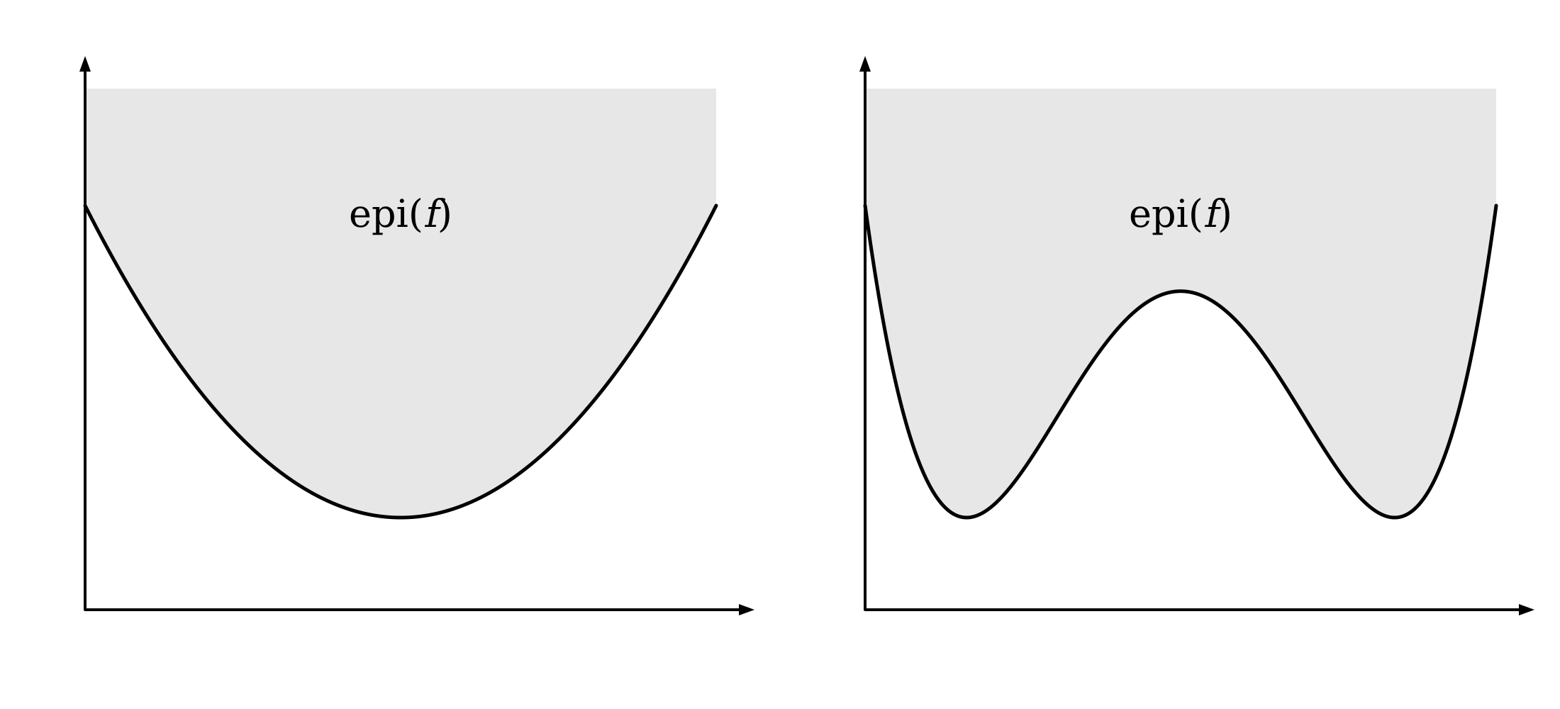
One possible way to define a convex function is a function whose epigraph is a convex set, like the one on the left in the image above. So now we shall find a relationship between the epigraph of \(f(\boldsymbol x, \boldsymbol y)\) and its partial minimization \(g(\boldsymbol x)\):
\[(\boldsymbol x, t) \in \operatorname{epi}(g) \\ \iff \\ g(\boldsymbol x) = \min_{\boldsymbol y} f(\boldsymbol x, \boldsymbol y) \leq t \\ \iff \\ \exists \boldsymbol y \quad f(\boldsymbol x, \boldsymbol y) \leq t \\ \iff \\ \exists \boldsymbol y \quad (\boldsymbol x, \boldsymbol y, t) \in \operatorname{epi}(f)\]In other words, the epigraph of \(g\) is just the projection of the epigraph of \(f\) onto the \((\boldsymbol x, t)\) coordinates - we take points \((\boldsymbol x, \boldsymbol y, t) \in \operatorname{epi}(f)\) and discard the \(\boldsymbol y\) part. Geometrically, it’s the shadow that the epigraph of \(f\) casts onto the \((\boldsymbol x, t)\) coordinates. Since \(\operatorname{epi}(f)\) is convex, so is the above projection, and thus \(g\) is convex. Visually, it looks like this - each slice of the epigraph of \(f\) becomes a vertical ray on the epigraph of \(g\).
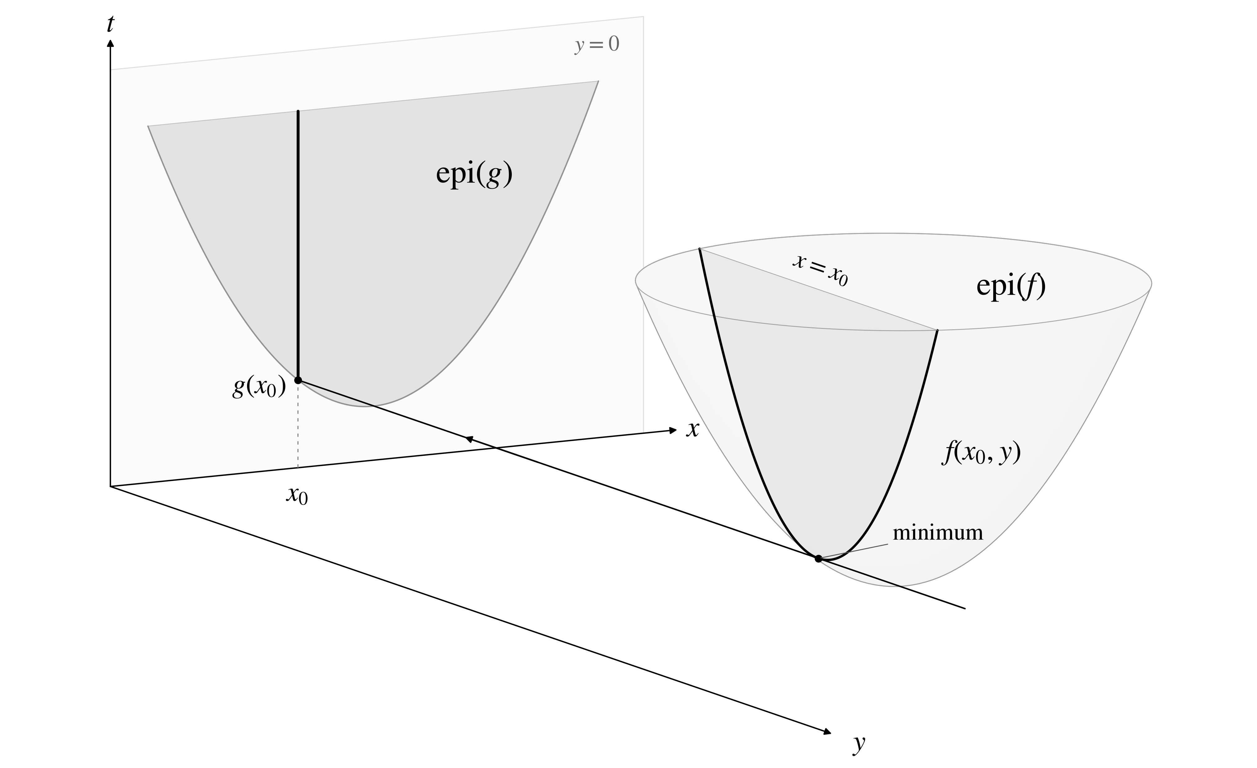
Now we can do some magic.
Why is the logistic loss convex?
In multi-class logistic regression we typically take the soft-max of the predictions and compute the cross-entropy loss w.r.t a one-hot encoding of the label. Doing some math, we have:
\[\operatorname{CrossEntropy}(\operatorname{softmax}(\boldsymbol u), \operatorname{one-hot}(i)) = \underbrace{\ln\left( \sum_{j=1}^n \mathrm{e}^{u_j} \right)}_{\operatorname{LogSumExp}(\boldsymbol u)} - u_i\]If we take a linear model \(\boldsymbol u = \boldsymbol W^T \boldsymbol x\), this is our friendly neighborhood linear logistic regression. When \(\boldsymbol u\) are token logits of our friendly neighborhood LLM, this is the pre-training loss of a single token. But essentially, both are just multi-class logistic regression losses.
In case of linear logistic regression, however, we can find a global optimum \(\boldsymbol W\), if it exists, because \(\operatorname{LogSumExp}\) is convex. Or so they say in the machine learning book. But if we look at these books or blogs on the Internet, various hairy formulas for its Hessian matrix are shown to be positive-semidefinite. Here we have an alternative path.
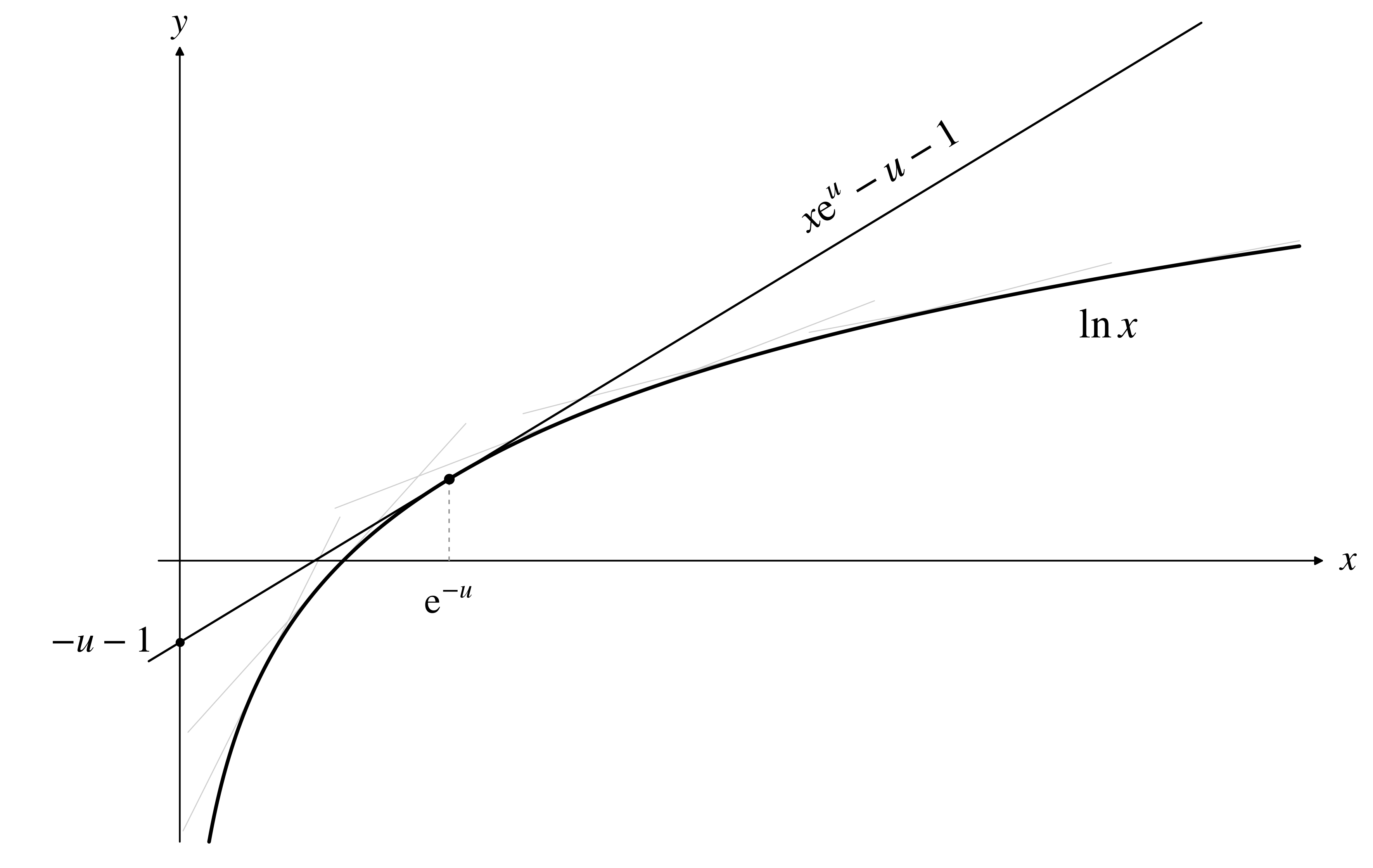
Turns out it is because we can write the logarithm as a minimum of functions:
\[\ln(x) = \min_u\left\{ x \mathrm{e}^u - u - 1 \right\}\]Why? Well, the logarithm is a concave function, so it is the minimum of all its tangents. And we have a very explicit way to characterize all the tangents - they all have a slope of \(e^{u}\) and an intercept of \(-u-1\). See the image:
So now that we have exposed the secret sauce, let’s see why \(\mathrm{LogSumExp}\) is convex:
\[\ln\left( \sum_{i=1}^n \mathrm{e}^{x_i} \right) = \min_u \left\{ e^u \sum_{i=1}^n \mathrm{e}^{x_i} - u - 1\right\}= \min_u \left\{ {\color{blue}\sum_{i=1}^n \mathrm{e}^{x_i + u} - u - 1}\right\} \tag{6}\]The blue term is a convex function of \((\boldsymbol x, u)\) - exponentials are convex, linear functions are convex, and a sum of two convex functions is convex. Consequently, its partial minimum over \(u\) is also convex. A one-line proof. No hairy Hessians and gradients, but requires knowing some elementary convex analysis.
But why is this proof interesting? Once we proved convexity, aren’t we done and we can just remember that this function is convex? Why do we care if the proof was hairy or not? So apparently this \(\mathrm{LogSumExp}\)-as-minimum trick is useful in many contexts, and next we shall look at one of those - learning to rank.
Simplifying learning to rank
When we learn to rank items, we are given a training set of previous lists of items shown to users, and the items the user liked. Assume for simplicity that the user liked one item in each list. When I say “liked” it can be anything indicating affinity, such as a click, a purchase, or whatever action we deem as “liking”. In this setting, our aim is learning a model that predicts higher scores for items that are more likely to be liked. We use these scores at inference to sort items before presenting them to the user. Thus, the scores have no meaning - only the order they induce has a meaning.
In this setting our data is a set of item lists, each item with its own features, and a binary label saying if it was liked. The lists, however, do not have to be all of the same size. So visually, our training set looks like this:
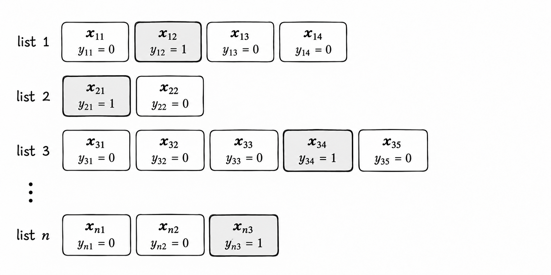
Our objective is learning a model \(s(\boldsymbol x)\) producing a score for each item, such that liked items get higher scores than those that were not liked. A famous way of doing so is treating the scores in each list as the logits of a categorical distribution, and just using the cross-entropy loss5. Thus, each row is a training sample whose loss is:
\[\ell_i(s)=-\sum_{j=1}^{n_i} y_{ij} \ln\left( \frac{\mathrm{e}^{s(\boldsymbol x_{ij})}}{\sum_{k=1}^{n_i} \mathrm{e}^{s(\boldsymbol x_{ik})}} \right) = \mathrm{LogSumExp}(s(\boldsymbol x_{i,1}), \ldots,s(\boldsymbol x_{i,n_i})) - \sum_{j=1}^{n_i} y_{ij} s(\boldsymbol x_{i, j}).\]Here we shall see an interesting trick - rather than eliminating a variable using partial minimization, we actually introduce a variable by formulating the \(\mathrm{LogSumExp}\) function as a partial minimum to gain a simplification. But to see what we are going to simplify, we need to understand what kind of complications we have here.
First, in many cases we would like to give higher importance to items occurring at the beginning of the list. This is, for example, because the users tend to look at them first and may not even look at later items at all. It is not obvious how to correctly do it here - if we had a loss function for each item separately, we could do some weighting. Moreover, from the intuition above we understand that a positive item at the beginning of the list is actually less informative than a positive item at the end - if the user really liked an item at the end, it probably stood out. We can think of various heuristics, but this is what they are - heuristics.
Another complication is that of data layout. Working with a constant mini-batch size of \(B\) lists doesn’t mean each mini-batch has the same number of items, since each list may have a different size. But we are computing a forward pass for \(s(\boldsymbol x)\) for every item separately. Finally, even if our model \(s\) is linear, and thus the entire learning problem is a convex optimization problem, using a convex solver framework such as CVXPY requires organizing the data nicely into a matrix. And we can’t - each row has a different number of items! We could pad, but the padding hack has its own complications and quirks, since the right padding is negative infinity (since \(\exp(-\infty) = 0\)), but this introduces its own challenges, both in frameworks like PyTorch and in CVXPY.
So now comes our partial minimization to the rescue! The loss can be equivalently written as:
\[\ell_i(s)=\mathrm{LogSumExp}(s(\boldsymbol x_{i,1}), \ldots,s(\boldsymbol x_{i,n_i})) - \sum_{j=1}^{n_i} y_{ij} s(\boldsymbol x_{i, j}),\]Using equation (6), we can write it as
\[\begin{align*} \ell_i(s) &=\min_{u_i} \left\{ \sum_{j=1}^{n_i}\mathrm{e}^{u_i+s(\boldsymbol x_{i,j})} - u_i - 1\right\} - \sum_{j=1}^{n_i} y_{i,j} s(\boldsymbol x_{i, j}), \\ &= \min_{u_i} \left\{ \sum_{j=1}^{n_i} \left(\mathrm{e}^{u_i+s(\boldsymbol x_{i,j})}- y_{ij} s(\boldsymbol x_{i,j})\right) - u_i - 1 \right\} \\ &= \min_{u_i} \left\{ \sum_{j=1}^{n_i} \left(\mathrm{e}^{u_i+s(\boldsymbol x_{i,j})}- y_{ij} s(\boldsymbol x_{i,j}) - \frac{u_i + 1}{n_i}\right) \right\} \\ \end{align*}\]The second line stems from the fact that the terms \(y_{i,j} s(\boldsymbol x_{i, j})\) do not depend on \(u_i\), and we can put any constant from outside the minimum to inside the minimum. The last line is just splitting an equal portion of \(-u_i-1\) between the items. So the problem of minimizing the loss over the entire training set can be written as:
\[\begin{align*} \min_s \left\{\sum_{i=1}^m \ell_i(s) \right\} &= \min_s \left\{ \sum_{i=1}^m \min_{u_i} \left\{ \sum_{j=1}^{n_i} \left(\mathrm{e}^{u_i+s(\boldsymbol x_{i,j})}- y_{ij} s(\boldsymbol x_{i,j}) - \frac{u_i + 1}{n_i} \right) \right\} \right\} \\ &= \min_{s, \boldsymbol u} \left\{ \sum_{i=1}^m \sum_{j=1}^{n_i} \left(\mathrm{e}^{u_i+s(\boldsymbol x_{i,j})}- y_{ij} s(\boldsymbol x_{i,j}) - \frac{u_i + 1}{n_i}\right) \right\} \end{align*}\]Now behold - we are minimizing a sum of functions of individual items rather than a sum of functions of entire lists. The price is adding an additional variable \(u_i\) for every list, for expressing its \(\mathrm{LogSumExp}\) function. So item \(j\) of list \(i\) gets the loss function:
\[\hat{\ell}_{ij}(s, u_i) = \mathrm{e}^{u_i+s(\boldsymbol x_{i,j})}- y_{ij} s(\boldsymbol x_{i,j}) - \frac{u_i + 1}{n_i}\]What we did was inflate the dimension of the optimization problem to get rid of the direct coupling between the list items - now we need to learn both the parameters of our scoring model \(s\) and the value of \(u_i\). Visually, it looks like this:
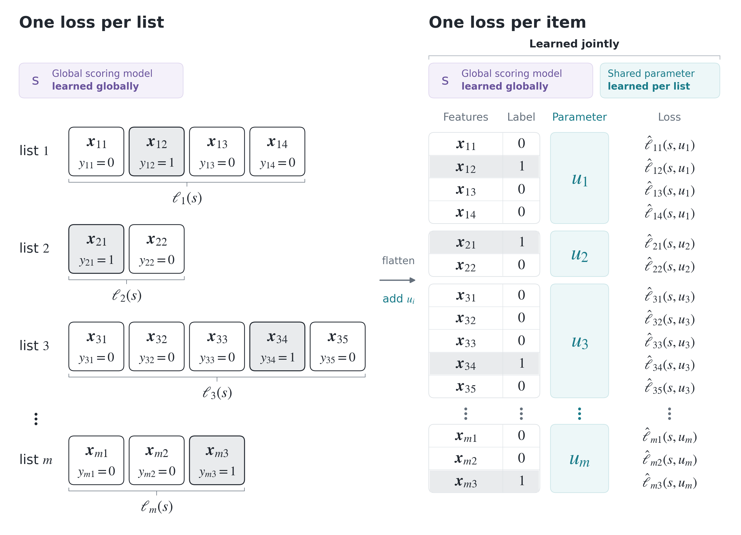
From the perspective of the learning algorithm, \(u_i\) is just another parameter to be learned. But of course, we know it’s there just as an auxiliary variable - after training, we only need the model \(s\). In PyTorch, it looks something like this:
import torch
from torch import nn
from torch.utils.data import DataLoader, TensorDataset

# Assume we're given:
#   X: (N, d) item features
#   y: (N,) binary labels, one positive per list
#   list_id: (N,) the index of the list each row of X belongs to, numbered 0, ..., m-1
loader = DataLoader(
    TensorDataset(X, y, list_id),
    batch_size=256,
    shuffle=True,
)

sizes = torch.bincount(list_id).to(dtype=torch.float32)
u = nn.Parameter(-torch.log(sizes)) # -log(n_i) is the optimal u when all scores are zero.
net = create_my_super_duper_cool_SOTA_network()

optimizer = torch.optim.Adam([*net.parameters(), u], lr=1e-3)
for epoch in range(20):
    for xb, yb, ids in loader:
        optimizer.zero_grad()

        scores = net(xb).reshape(-1)
        item_losses = torch.exp(ui + scores) - yb * scores - (ui + 1) / sizes[ids]
        loss = item_losses.mean()

        loss.backward()
        optimizer.step()
If \(s\) is linear, the problem becomes convex, and we can even use a standard convex solver provided that the dataset is not huge. Here is a CVXPY example that works if our dataset has a few tens of thousands of examples. Nice for prototypes:
import numpy as np
import cvxpy as cp

# Assume we're given:
#   X: (N, d) item features
#   y: (N,) binary labels, one positive per list
#   list_id: (N,) the index of the list each row of X belongs to, numbered 0, ..., m-1

sizes = np.bincount(list_id)
w = cp.Variable(X.shape[1])  # Global parameters of the linear model <w, x>
u = cp.Variable(len(sizes))  # One parameter per list

scores = X @ w
ui = u[list_id]  # Share each u_i across its list

item_losses = (
    cp.exp(ui + scores) - cp.multiply(y, scores) - cp.multiply(1.0 / sizes[list_id], ui + 1)
)
problem = cp.Problem(cp.Minimize(cp.sum(item_losses)))
problem.solve()
Doing this with cvxpy.log_sum_exp where the size of each list is variable would cause a HUGE overhead - due to their variable size, we’d have to manually iterate over the lists and compute the log-sum-exp terms for each item. But the flattening, both for PyTorch and for CVXPY, allows us to treat the data as one big array of items having individual losses.
In real recommender systems, not all item positions are equally exposed to users. Users typically see the first item, the second is observed slightly less, and so on. This is called exposure bias - the user is exposed less to later items in a list. This is typically modeled by the probability of observing the item at position $j$ given that they observed the first item. Let’s denote those probabilities by \(p_1, \ldots, p_n\) for a list of \(n\) items, with \(p_1=1\) by definition.
Now let’s think intuitively. A click on the first or second item may be informative, but a click on the 8th is much more so - it means that this item, that the user rarely even sees, stood out. Conversely, a skip of a top item is informative - it means that the user saw it and chose to skip it, but a skip on a later item is less so, since it may be the case that the user hasn’t even looked at it. Now let’s look at our item-wise loss for a fixed \(u_i\) as a function of the score \(s(\boldsymbol x_j)\):
\[\hat{\ell}_{ij}(s, u_i) = \underbrace{\mathrm{e}^{u_i+s(\boldsymbol x_{i,j})}}_{\text{high score penalty}}- \underbrace{y_{ij} s(\boldsymbol x_{i,j})}_{\text{click reward}} - \underbrace{\frac{u_i + 1}{n_i}}_{\text{const}}\]So intuitively, we would like to incur a higher penalty on higher items, without hurting their reward, meaning we can modify the loss as:
\[\hat{\ell}_{ij}(s, u_i)= {\color{blue} p_j} \mathrm{e}^{u_i+s(\boldsymbol x_{i,j})}- y_{ij} s(\boldsymbol x_{i,j}) - \frac{u_i + 1}{n_i}\]Now let’s see what it means for the entire list by eliminating \(u_i\) and getting a penalized version of the loss of the \(i\)-th list:
\[\begin{align*} \ell_i(s) &= \min_{u_i} \sum_{j=1}^{n_i} \hat{\ell}_{ij}(s, u_i) \\ &= \min_{u_i} \left\{ \sum_{j=1}^{n_i} p_j\mathrm{e}^{u_i+s(\boldsymbol x_{i,j})} - u_i - 1 \right\} - \sum_{j=1}^{n_i} y_{ij} s(\boldsymbol x_{ij}) \\ &= \operatorname{LogSumExp}(s(\boldsymbol x_{i,1}) + \ln(p_1), \ldots, s(\boldsymbol x_{i,n_i}) + \ln(p_{n_i})) - \sum_{j=1}^{n_i} y_{ij} s(\boldsymbol x_{ij}) \end{align*}\]This is equivalent to just adding \(\ln(p_j)\) to the score of each item at position \(j\)! The partial minimization trick let us first add an auxiliary variable to decompose the loss into a penalty and a reward, modify the penalty, and then eliminate the auxiliary variable to obtain a new exposure-adjusted loss for the entire list. Adding the exposure bias in this way exists in the literature in papers by Abeliuk et al.6 and Grant et al. 7, but it is just shown as a modeling assumption, without explaining why it makes sense. In other domains that are not learning to rank, this same formula has been derived from Bayes’ rule - see papers by Ren et al. 8 and Menon et al. 9. But I haven’t seen it derived anywhere from this perspective - decomposing the well-known loss from the literature into a penalty and a reward, and making sure that only the penalty is affected by the exposure probability to achieve the desired effect.
Summary
This post has a “theoretico-practical” smell - we use a theoretical tool, partial minimization, to simplify problems in two different ways. The first way is to eliminate variables to reduce dimensions or produce a tractable problem we can solve using standard computational tools. The second way is to actually introduce auxiliary variables and inflate the problem to simplify implementation or perform a theoretical analysis to derive new loss functions that serve our needs. I hope you enjoyed it, and it gave you new perspectives on machine learning algorithms that have an optimization-driven rather than probability-driven justification that we see everywhere.
References
-
Hastie, Trevor, Robert Tibshirani, and Andreas Buja. “Flexible discriminant analysis by optimal scoring.” Journal of the American statistical association 89.428 (1994): 1255-1270. ↩
-
Mairal, Julien, Francis Bach, and Jean Ponce. “Sparse modeling for image and vision processing.” Foundations and Trends in Computer Graphics and Vision 8.2-3 (2014): 85-283. ↩
-
Ding, Chris, et al. “Orthogonal nonnegative matrix t-factorizations for clustering.” Proceedings of the 12th ACM SIGKDD international conference on Knowledge discovery and data mining. 2006. ↩
-
Boyd, Stephen, et al. “Convex Optimization.” Cambridge University Press. 2004. ↩
-
Bruch, Sebastian, et al. “An analysis of the softmax cross entropy loss for learning-to-rank with binary relevance.” Proceedings of the 2019 ACM SIGIR international conference on theory of information retrieval. 2019. ↩
-
Abeliuk, Andrés, et al. “Assortment optimization under a multinomial logit model with position bias and social influence.” 4OR 14.1 (2016): 57-75. ↩
-
Grant, James A., and David S. Leslie. “Learning to rank under multinomial logit choice.” Journal of Machine Learning Research 24.260 (2023): 1-49. ↩
-
Ren, Jiawei, et al. “Balanced meta-softmax for long-tailed visual recognition.” Advances in neural information processing systems 33 (2020): 4175-4186. ↩
-
Menon, Aditya Krishna, et al. “Long-Tail Learning via Logit Adjustment.” International Conference on Learning Representations, 2021, openreview.net/forum?id=37nvvqkCo5. ↩