When Eigenvalues Collide

Intro

Up until now in the series we discussed mainly the expressive power of different variants of our model family,

\[f({\boldsymbol x};{\boldsymbol A}_{0..n}) = \lambda_k \Bigl({\boldsymbol A}_0 + \sum_{i=1}^n x_i {\boldsymbol A}_i\Bigr),\]

where each \(\boldsymbol A_i\) is a symmetric matrix. In this post we tackle a different angle - the speed of learning from data.

The optimization literature is full of results on the rate of convergence under various assumptions, but on one thing there is a clear concensus - the rate of convergence of an optimization algorithm in general, and a model training algorithm in particular, heavily depends on the sensitivity of the cost function or its gradient to changes.

When training a model we minimize the average loss over the training set - so the cost we minimize, as a function of the parameters, is composed of the model itself and the loss function we use. Thus, if our model’s gradients change abruptly even under a small change of the model’s parameters, the gradients of the entire cost function inherit this behavior.

So in this post we shall study, what makes gradients change abruptly and apply an unusual tool from optimization, Moreau envelopes, to make the above \(f\) better behaved for training. Of course, we aren’t stopping at theory. We shall derive a closed-form formula for a better behaved variant of our model using Moreau envelopes, and shall have plenty of code and plots to demonstrate a significantly improved training behavior. Thus, this post is going to be both math and code heavy, so brace yourselves!

Stochastic optimization theory for beginners

From a theoretical perspective, (supervised) training is formulated as minimizing the expected loss:

\[L({\boldsymbol A}_{0..n}) = \operatorname*{\mathbb{E}}_{\boldsymbol x, y}\,\left[\ell(f({\boldsymbol x};{\boldsymbol A}_{0..n}), y) \right]\]

We minimize \(L\) by repeatedly obtaining a vector \(\boldsymbol g\) whose expectation is \(\nabla L\), such as the loss gradient of the currently sampled mini-batch. The vectors \(\boldsymbol g\) at each step can be thought of as an approximation of the full gradient of \(L\).

The speed of convergence, be it plain stochastic gradient descent or some fancy optimizer, typically depends on two factors:

1. How do the loss gradients change as model parameters change, i.e., a Lipschitz constant of the loss gradients;
2. How do the loss gradients vary as we sample different mini-batches, i.e., the 2ⁿᵈ moment.

Since our model is the \(k\)-th smallest eigenvalue of the matrix \({\boldsymbol A}_0 + \sum_{i=1}^n x_i {\boldsymbol A}_i\), which depends linearly on both the model parameters and the features, both questions boil down to one key question:

How does the derivative of \(\lambda_k(\boldsymbol W)\) vary as \(\boldsymbol W\) varies?

There are also variants of these aspects for nondifferentiable functions, but our intent here is to keep the discussion simple at this stage. So let’s study some answers the literature provides to the variation of eigenvalue derivatives.

A tale of colliding eigenvalues

The \(k\)-th eigenvalue \(\lambda_k(\boldsymbol W)\) has a corresponding normalized eigenvector \(\boldsymbol{v}_k(\boldsymbol W)\). As we pointed out in a previous post, we have:

\[\nabla \lambda_k(\boldsymbol W) = \boldsymbol{v}_k(\boldsymbol W) \boldsymbol{v}_k(\boldsymbol W)^T.\]

We know that the normalized eigenvector is not unique. For example, if \(\boldsymbol v\) is an eigenvector, so is \(- \boldsymbol v\). Sign, of course, is not a problem - the gradient is well-defined because the sign cancels out in the product above. But there might also be an entire subspace of eigenvectors due to multiplicities. As we discussed, this yields a set of derivatives - the Clarke sub-differential, which is a set of generalized derivatives useful for learning.

So the question we are dealing here is - what can we say about \(\| \nabla \lambda_k(\boldsymbol W) - \nabla \lambda_k(\boldsymbol W + \boldsymbol \Delta)\|\) as a function of \(\| \boldsymbol \Delta \|\)? To simplify discussion, we assume that our eigenvalue has multiplicity 1, and thus we have a regular gradient. Turns out a central object is the eigenvalue gap:

\[\mathrm{gap}_{k,j}(\boldsymbol W) = \lambda_k(\boldsymbol W) - \lambda_j(\boldsymbol W)\]

You can probably guess that small gaps mean “ill-behaved”, and large gaps are “well-behaved”. In the limit, when the gap is zero, the eigenvalues “collide” and we have a multiplicity. In this case the “ill-behavior” is at its maximum - there is no gradient, and we have a Clarke sub-differential set.

The Davis Kahan theorem

The celebrated Davis-Kahan theorem¹ imposes a bound on the angle between eigenvector spaces of two nearby matrices. The theorem relies on the smallest eigenvalue gap: \(\operatorname{min-gap}_{k}(\boldsymbol W) = \min_{j \neq k} |\mathrm{gap}_{k,j}(\boldsymbol W)|\) It is written generally, but in practice if we aren’t dealing with neither the smallest nor the largest eigenvalue, the gap is \(\operatorname{min-gap}_{k}(\boldsymbol W) = \min\left( \mathrm{gap}_{k+1,k}(\boldsymbol W), \mathrm{gap}_{k,k-1}(\boldsymbol W) \right),\) i.e, the gap between our desired eigenvalue and the closest one above or below it.

In its full glory, the Davis-Kahan theorem covers the case of eigenvalues with multiplicities, but here is a simplified version, and written in the terminology we adopted in this post:

Let \(\boldsymbol W\) and \(\boldsymbol \Delta\) be two symmetric matrices. Suppose that the eigenvalues \(\lambda_k(\boldsymbol W), \lambda_k(\boldsymbol W + \boldsymbol \Delta)\) are simple. Then, \(\|\nabla \lambda_k(\boldsymbol W) - \nabla \lambda_k(\boldsymbol W + \boldsymbol \Delta) \|_2 \leq \frac{\|\boldsymbol \Delta \|_2}{\operatorname{min-gap}(\boldsymbol W) }\)

So even two nearby matrices can have very different eigenvalue function gradients if the eigenvalue gap is small. Of course, for very small gaps the bound is vacuous, this is because \(\|\nabla \lambda_k(\boldsymbol W)\|_2 \leq 1\). And it’s only an upper bound. But it gives us a rough idea of what is going on - eigenvalue gaps play a role in gradient stability. But it’s also global - it doesn’t require the \(\boldsymbol \Delta\) to be infinitesimally-small.

The first-order approximation

In contrast to Davis Kahan, now we present a local result that holds in a small neighborhood of our function argument \(\boldsymbol W\), but provides a slightly different insight - now it’s not an upper bound, but a first order approximation. Let me first present the result:

Let \(\boldsymbol \phi(t) = \nabla \lambda_k(\boldsymbol W + t \boldsymbol \Delta)\), and assume that \(\lambda_j(\boldsymbol W)\) is a simple eigenvalue with a corresponding eigenvector \(\boldsymbol v_j\) for all \(j\).

Then, \(\nabla \boldsymbol \phi(t) = \sum_{j \neq k} \frac{(\boldsymbol v_j^T \boldsymbol \Delta \boldsymbol v_k) \boldsymbol v_j \boldsymbol v_k^T + (\boldsymbol v_k^T \boldsymbol \Delta \boldsymbol v_j) \boldsymbol v_k \boldsymbol v_j^T}{\mathrm{gap}_{k,j}(\boldsymbol W)}\)

The above is a simplification of a more general eigenvector perturbation result, a well known result described by Kato², and more nicely presented in the “First-order perturbation theory for eigenvalues and eigenvectors”³.

Let’s first understand what the theorem says. Note that \(\boldsymbol \phi\) is our desired gradient of the eigenvalue function along the line starting at \(\boldsymbol W\) in the direction \(\boldsymbol \Delta\). So the derivative \(\nabla \boldsymbol \phi\) represents the local rates of change in this direction.

Here we also see that eigenvalue gaps play a key role in the denominator. Small gaps potentially add summands having a large norm. And here it is not just upper bound - it is a direct equality, but it’s local in nature. It measures the rate of change only in an infinitesimal neighborhood of \(\boldsymbol W\), but it also shows us that the rate of change may actually be inversely-proportional to the gaps and it’s not only a loose upper bound.

Towards a solution

So can we somehow make sure our matrices never have small eigenvalue gaps around the mid eigenvalue? Personally - I don’t know how. But perhaps we can try something else, like averaging nearby eigenvalues? Having one eigenvalue with small gaps is likely, but having several at once with small gaps is much less likely!

But here is the problem - how would we know how many eigenvalues to average, and what weight should we give to each eigenvalue? Turns out a remedy comes from my favorite subject - convex analysis. We can smooth out eigenvalue functions in a controlled and rigorous manner, and quite easily implement the idea in code.

KyFan and Moreau entered the chat

For describing the smoothing technique, it will be convenient talking about the \(r\)-th largest eigenvalue of a matrix, which we denote by \(\mu_r(\boldsymbol W)\). Of course, both views are equivalent, since for an \(n \times n\) matrix we have

\[\lambda_k(\boldsymbol W) = \mu_{n - k + 1}(\boldsymbol W).\]

Recall from our post on interpreting the model family, that the sum of the \(r\) largest eigenvalues,

\[M_r(\boldsymbol W) = \sum_{j=1}^r \mu_j(\boldsymbol W),\]

is a convex function. Indeed, in that very post we saw that this largest eigenvalue sum function can be equivalently written using the Ky Fan Variational Principle, called after the Chinese-American mathematician Ky Fan:

\[M_r(\boldsymbol W) = \max_{\boldsymbol P} \left\{ \langle \boldsymbol P, \boldsymbol W \rangle : \operatorname{tr}(\boldsymbol P) = r, \boldsymbol P \succeq \boldsymbol 0, \boldsymbol I-\boldsymbol P \succeq 0 \right\}. \tag{M}\]

The notation \(\boldsymbol P \succeq \boldsymbol 0\) means that \(\boldsymbol P\) is a positive semi-definite matrix. The \(r\)-th largest eigenvalue is just a difference of these two convex functions:

\[\mu_r(\boldsymbol W) = M_r(\boldsymbol W) - M_{r-1}(\boldsymbol W).\]

So now that we’ve met Ky Fan, let’s meet Jean-Jaques Moreau and his Moreau envelope. In fact, this blog already introduced him in the proximal-point post series, but here we are going to see the envelope in a different form:

Let \(\phi(\boldsymbol u) = \max_{\boldsymbol v} \{ \langle \boldsymbol u, \boldsymbol v \rangle - \varphi(\boldsymbol v) \}\), where \(\varphi\) is a convex function, and let \(\alpha > 0\). Then the Moreau envelope of \(\phi\) is:

\[\tilde{\phi}_{\alpha}(\boldsymbol u) = \max_{\boldsymbol v} \{ \langle \boldsymbol u, \boldsymbol v \rangle - \varphi(\boldsymbol v) - \tfrac{\alpha}{2} \| \boldsymbol v \|_2^2 \} \tag{E}\]

Intuitively, we take a function defined as a maximum, and introduce quadratic regularization to the maximization problem that defines that function.

The first property that we immediately see is that it is indeed an “envelope”, meaning, the envelope of \(\phi\) is a lower bound for \(\phi\) itself, since we subtract a non-negative term inside the maximum.

But a more useful property, whose proof is out of the scope of this post, is that the Moreau envelope is always differentiable and smooth:

\[\| \nabla \tilde{\phi}_{\alpha}(\boldsymbol u) - \nabla \tilde{\phi}_{\alpha}(\boldsymbol u + \boldsymbol \delta) \|_2 \leq \frac{1}{\alpha} \| \boldsymbol \delta \|_2\]

This appears to be exactly the property we are looking for - the rate of change of its derivative is bounded by the size of the change up to a constant. Here we get a direct control over that constant - it is at most \(\tfrac{1}{\alpha}\).

Finally, we have an explicit formula for the gradient. You wouldn’t be surprised - it’s just the maximizer of the maximization problem that defines the envelope:

\[\nabla \tilde{\phi}_{\alpha}(\boldsymbol u) = \operatorname*{argmax}_{\boldsymbol v} \left \{ \langle \boldsymbol u, \boldsymbol v \rangle - \varphi(\boldsymbol v) - \tfrac{\alpha}{2} \| \boldsymbol v \|_2^2 \right\}.\]

So why is this object useful for our case? Because we can write eigenvalues using such a “max” formulation!

But here we are at luck! The Ky Fan principle lets us write the sum of the \(r\) largest eigenvalues exactly in the form we need - as a max function. Its Moreau envelope let us produce a controlled smooth approximation.

Here is our plan. We shall devise a closed-form solution for the Moreau envelope \(\tilde{M}_{r,\alpha}\) of the sum of \(r\)-th largest eigenvalues function \(M_r\). This, in turn, leads to a smooth approximation of the \(r\)-th largest eigenvalue: \(\tilde{\mu}_{r,\alpha} = \tilde{M}_{r,\alpha} - \tilde{M}_{r-1,\alpha}\) Then, we shall implement it in Python, study it by plotting and train a model on the California Housing dataset to observe improved convergence rate.

As we shall soon see, this smooth approximation is just a weighted average of a window of eigenvalues around the \(r\)-th, but with carefully chosen weights.

Moreau envelope of \(M_r\)

Taking the \(M_r\) as formulated in equation (M) and applying the Moreau envelope formula in equation (E), we have

\[\tilde{M}_{r, \alpha}(\boldsymbol W) = \max_{\boldsymbol P} \left\{ \langle \boldsymbol P, \boldsymbol W \rangle - \frac{\alpha}{2} \| \boldsymbol P \|_F^2 : \boldsymbol P \succeq \boldsymbol 0, \boldsymbol I-\boldsymbol P \succeq 0, \operatorname{tr}(\boldsymbol P) = r \right\},\]

where \(\| \boldsymbol P \|_F^2\) is is just the sum of the squares of the matrix entries, known as the squared Frobenius norm. At first glance this appears like a hard to solve optimization problem - a quadratic cost, and a matrix with a positive semidefinite constraint.

But it turns out there is a trick. The Frobenius norm turns out to be invariant to multiplication by an orthogonal matrix. Take the eigenvalue decomposition

\[\boldsymbol W = \boldsymbol U \boldsymbol M \boldsymbol U^T,\]

with a diagonal matrix of eigenvalues \(\boldsymbol M\) and an orthogonal matrix of eigenvectors \(\boldsymbol U\). Since any similarity transformation preserves eigenvalues. So, via the change of variables \(\boldsymbol Q = \boldsymbol U \boldsymbol P \boldsymbol U^T\), we can write:

\[\begin{aligned} \tilde{M}_{r, \alpha}(\boldsymbol W) &= \max_{\boldsymbol P} \left\{ \langle \boldsymbol P, \boldsymbol W \rangle - \frac{\alpha}{2} \| \boldsymbol P \|_F^2 : \boldsymbol P \succeq \boldsymbol 0, \boldsymbol I - \boldsymbol P \succeq 0, \operatorname{tr}(\boldsymbol P) = r \right\} \\ &= \max_{\boldsymbol Q} \left\{ \langle \boldsymbol Q, \boldsymbol M \rangle - \frac{\alpha}{2} \| \boldsymbol Q \|_F^2 : \boldsymbol Q \succeq \boldsymbol 0, \boldsymbol I - \boldsymbol Q \succeq 0, \operatorname{tr}(\boldsymbol Q) = r \right\}. \end{aligned}\]

It appears that \(\boldsymbol W\) has disappeared from the maximization problem - it has not. The matrix \(\boldsymbol M\) is a function of \(\boldsymbol W\) - it contains its eigenvalues.

Now, since \(\boldsymbol M\) is just the diagonal matrix of eigenvalues with \(\boldsymbol \mu = \operatorname{diag}(\boldsymbol M)\), the off-diagonal entries of \(\boldsymbol Q\) do not matter and can be set to zero. We’re left with an optimization problem over the vector \(\boldsymbol q = \operatorname{diag}(\boldsymbol Q)\):

\[\tilde{M}_{r, \alpha}(\boldsymbol W) = \max_{\boldsymbol q} \left\{ \langle \boldsymbol q, \boldsymbol \mu(\boldsymbol W) \rangle - \frac{\alpha}{2} \| \boldsymbol q \|_2^2 : 0 \leq q_j \leq 1, \sum_j q_j = r \right\}\]

This is progress! The optimization problem is now on vectors instead of matrices. The final trick up our sleeve is recognizing this problem as exactly the projection onto a simplex, and has a readily available algorithm. Indeed, by square completion we have:

\[\langle \boldsymbol q, \boldsymbol \mu(\boldsymbol W) \rangle - \frac{\alpha}{2} \| \boldsymbol q \|_2^2 = - \frac{\alpha}{2} \| \boldsymbol q - \frac{1}{\alpha} \boldsymbol \mu(\boldsymbol W) \|_2^2 + \frac{1}{\alpha} \|\boldsymbol \mu(\boldsymbol W)\|_2^2.\]

Since \(\frac{1}{\alpha} \|\boldsymbol \mu(\boldsymbol W)\|_2^2\) does not depend on \(\boldsymbol q\) we can “pull it out” of the optimization problem, and obtain:

\[\tilde{M}_{r, \alpha}(\boldsymbol W) = -\frac{\alpha}{2}\min_{\boldsymbol q} \left\{ \| \boldsymbol q - \frac{1}{\alpha} \boldsymbol \mu(\boldsymbol W) \|_2^2 : 0 \leq q_j \leq 1, \sum_j q_j = r \right\} + \frac{1}{\alpha} \|\boldsymbol \mu(\boldsymbol W)\|_2^2.\]

Note, that the \(\max\) turned to a \(\min\) because we pulled out the negative term \(-\frac{\alpha}{2}\) out of the optimization problem. Now, looking at the \(\min\) we can recognize the projection - it’s the closest vector to \(\frac{1}{\alpha} \boldsymbol \mu(\boldsymbol W)\) that satisfies the capped \(r\)-simplex constraints - its entries are between 0 and 1, and sum to \(r\).

Having solved for \(\boldsymbol q\), which if you recall originated from the change of variable, we can recover \(\boldsymbol P\) using exactly the formula we used for the change of variable, as \(\boldsymbol P = \boldsymbol U \boldsymbol Q \boldsymbol U^T\), where \(\boldsymbol Q\) is a diagonal matrix with \(\boldsymbol q\) in its diagonal.

So the algorithm for computing \(\tilde{M}_{r, \alpha}(\boldsymbol W)\) and its gradient is quite simple:

1. Compute the spectral decomposition \(\boldsymbol W = \boldsymbol U \boldsymbol M \boldsymbol U^T\).
2. Let \(\boldsymbol \mu = \operatorname{diag}(\boldsymbol M)\), and project \(\frac{1}{\alpha} \boldsymbol \mu\) onto the capped \(r\)-simplex to obtain \(\boldsymbol q^*\).
3. Output:
   1. Value: \(\tilde{M}_{r, \alpha}(\boldsymbol W) = \langle \boldsymbol q^*, \boldsymbol \mu\rangle - \frac{\alpha}{2} \| \boldsymbol q^* \|_2^2\)
   2. Gradient: \(\nabla \tilde{M}_{r, \alpha}(\boldsymbol W) = \boldsymbol U \boldsymbol Q \boldsymbol U^T = \sum_j q_j \boldsymbol U_{:, j} \boldsymbol U_{:, j}^T\)

Here I used the Python notation \(\boldsymbol U_{:, j}\) to denote the \(j\)-th column of \(\boldsymbol U\), and \(\boldsymbol Q\) is the diagonal matrix with diagonal \(\boldsymbol q\).

Now let’s handle the “ project onto the capped \(r\)-simplex” step, which is our final obstacle towards a Python implementation. This one final step towards an implementable algorithm requires some explaining, and this is where we begin coding. We shall do it bottom-up - implement simplex projection, then implement and study \(\tilde{M}_{r, \alpha}(\boldsymbol W)\), and finally use it to implement and use it for a smooth approximation of the \(r\)-th largest eigenvalue.

Projecting onto the capped simplex

So our objective is solving an optimization problem of the form

\[\min_{\boldsymbol q} \left\{ \| \boldsymbol q - \boldsymbol y \|_2^2 :0 \leq q_j \leq 1, \sum_j q_j = r \right\} \tag{P}\]

I will not dig into the derivation of the algorithm, since this post is already math heavy and this would be a large detour. So I’ll just present one well-known approach⁴, and focus on the computational aspect, rather than explaining why it is the projection.

The optimal vector \(\boldsymbol q^*\) is obtained by

\[q_i^* = \operatorname{clip}(y_i + \nu, 0, 1),\]

where \(\operatorname{clip}(z, a, b)\) clips \(z\) to lie in the interval \([a, b]\), and \(\nu\) is a solution of the univariate equation

\[\sum_i \operatorname{clip}(y_i + \nu, 0, 1) = r. \tag{Q}\]

In other words, the projection of \(\boldsymbol y\) is obtained by shifting all coordinates a constant \(\nu\) and clipping to \([0, 1]\), which is chosen such that the clipped coordinates sum to \(r\). So the main computational challenge is solving this equation and finding the “shift” \(\nu\).

We shall begin by studying the left-hand side of the equation as a function of \(\nu\). First, note that

\[\operatorname{clip}(z, 0, 1) = \operatorname{relu}(z) - \operatorname{relu}(z - 1),\]

and therefore the left-hand side can be written as

\[\sum_i \operatorname{relu}(y_i + \nu) - \sum_i \operatorname{relu}(y_i - 1 + \nu) = r.\]

Since \(\operatorname{relu}(a + \nu)\) is a piecewise linear function with one break point at \(\nu=-a\), we conclude that the left-hand side is a piecewise linear function with break-points at \(-y_i\) and \(1 - y_i\). Moreover, since \(\operatorname{clip}(y_i + \nu, 0, 1)\) is a non-decreasing function of \(\nu\), the left-hand side must be non-decreasing.

Let’s get convinced by plotting. Here is a simple NumPy implementation of the left-hand side:

import numpy as np

def capped_simplex_lhs(ys, nus):
    return np.sum(
        np.clip(ys[np.newaxis, ...] + nus[..., np.newaxis], 0, 1),
        axis=-1
    )

Now let’s plot the function with \(\boldsymbol y = (-2, -0.5, 0, 2)\) on the domain \([-4, 4]\), and plot the break points at \(-y_i\) and \(1 - y_i\) as vertical lines:

import matplotlib.pyplot as plt

ys = np.array([-2, -0.5, 0, 2])
nus = np.linspace(-4, 4, 1000)
plt.plot(nus, capped_simplex_lhs(ys, nus), color='blue')
for y in ys:
    plt.axvline(-y, linestyle='dotted', linewidth=0.5, color='black')
    plt.axvline(1 - y, linestyle='dotted', linewidth=0.5, color='black')
plt.axhline(2, color='red', linestyle='--')
plt.show()

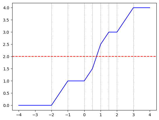
Indeed, we can see that the function changes slope exactly at the break points denoted by the vertical lines, and is non-decreasing. I also plotted a horizontal line to simulate a right-hand side of \(r=2\) in the equation in red. The solution is obtained where the blue and the red lines intersect.

Since the function is non-decreasing we can of course compute the solution using simple binary search. But there is a direct method - we compute the coefficients of the linear functions between each two break-points, intersect each one with the red line, and if the intersection falls in the interval - viola, we found it!

So let’s begin by computing the coefficients. To that end, the difference of ReLU functions view is useful. Each break-point \(-y_i\) originates from the term \(\mathrm{relu}(y_i + \nu)\). It is zero to the left of the break-point, and a linear function with slope \(1\) and intercept \(y_i\) to the right. The break-point \(1 - y_i\) originates from the term \(-\mathrm{relu}(y_i - 1 + \nu)\), which is zero to the left of the break-point, and a linear function with slope -1 and intercept \(1-y_i\). Thus, if we “traverse” the \(\nu\) axis from left to right, we begin with the zero function, which has slope and intercept zero, and each break-point we encounter adds a corresponding slope and intercept.

To construct the coefficients we need to sort the break-points, and compute a cumulative sum vector of the corresponding slopes, and another one of the corresponding intercepts.

def capped_simplex_coefficients(y):
    """Return breaks, intercepts, and slopes for the piecewise-linear function

        f(x) = sum_j clip(y_j + x, 0, 1).

    On each interval between two breaks,

        f(x) = intercept + slope * x.
    """
    *B, N = y.shape

    # break points and slope contribution + bias contribution at each point
    breaks = np.concatenate([-y, 1 - y], axis=-1)
    slope_step = np.concatenate([np.ones_like(y), -np.ones_like(y)], axis=-1)
    intercept_step = np.concatenate([y, 1 - y], axis=-1)

    # sort all arrays by break points
    order = np.argsort(breaks, axis=-1)
    breaks = np.take_along_axis(breaks, order, axis=-1)
    slope_step = np.take_along_axis(slope_step, order, axis=-1)
    intercept_step = np.take_along_axis(intercept_step, order, axis=-1)

    # create coefficiens of all linear functions
    slopes = np.cumsum(slope_step, axis=-1)
    intercepts = np.cumsum(intercept_step, axis=-1)

    return breaks, slopes, intercepts

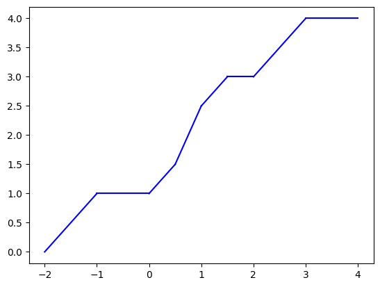
Let’s plot it:

breaks, slopes, intercepts = capped_simplex_coefficients(ys)

intervals = np.r_[breaks, 4]
for frm, to, slp, intr in zip(intervals[:-1], intervals[1:], slopes, intercepts):
    xs = np.linspace(frm, to, 100)
    plt.plot(xs, slp * xs + intr, color='blue')
plt.show()

Now how do we solve the equation (Q) in practice? We look at the function values at the break-points, look for the first one that is at least \(r\) - this is our “hit” and its index denotes the interval. Then, we just solve a linear equation in that interval.

So let’s try it out:

r = 2

break_vals = breaks * slopes + intercepts
hit = np.argmax(break_vals >= r, axis=-1)  # index of first break valued below m
intr_idx = np.maximum(hit - 1, 0)          # index of interval = one before first hit
sol_x = (r - intercepts[intr_idx]) / slopes[intr_idx]

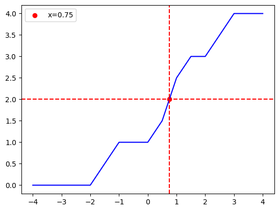
To see that we hit the solution, here is a plot of the left-hand side function, the right-hand side, and the solution itself:

xs = np.linspace(-4, 4, 1000)
plt.plot(xs, capped_simplex_lhs(ys, xs), color='blue') # LHS
plt.axhline(r, color='red', linestyle='--')            # RHS
plt.axvline(sol_x, color='red', linestyle='--')
plt.scatter(sol_x, r, color='red', label=f'x={sol_x:.2f}')
plt.legend()

Very nice! Now to do it in a vectorized manner over a mini-batch of such equations, we need to take some more care with indexing. But the formula remains the same. There is one edge-case we also need to take care of - a zero slope. In this case, if we “hit” an interval with a zero slope, it means we can take any point in that interval as our solution. So we choose to take the left break-point. Here is the code that takes care for both indexing and the edge case:

def _gather_last(a: np.ndarray, index: np.ndarray) -> np.ndarray:
    return np.take_along_axis(a, index[..., None], axis=-1)[..., 0]

def solve_piecewise_linear(r, breaks, slopes, intercepts):
    value_at_breaks = intercepts + slopes * breaks

    hit = np.asarray(np.argmax(value_at_breaks >= r, axis=-1))
    intr_idx = np.maximum(hit - 1, 0)

    intercepts = _gather_last(intercepts, intr_idx)
    slopes = _gather_last(slopes, intr_idx)
    breaks = _gather_last(breaks, intr_idx)

    return np.divide(
        r - intercepts, slopes,
        out=np.array(breaks, copy=True),
        where=slopes != 0,
    )

As a sanity test, let’s see that it works for our one equation:

solve_piecewise_linear(r, breaks, slopes, intercepts)

array(-0.75)

Indeed, the same solution we’ve just seen visually in the plot.

Now we get back to projecting onto the simplex. Recall that the equation gives us the correct amount of shift, and the projection is done by shifting and clipping. We do it, again, in a vectorized manner to project an entire mini-batch of points:

def project_onto_capped_simplex(ys, r):
    breaks, slopes, intercepts = capped_simplex_coefficients(ys)
    x_sol = solve_piecewise_linear(r, breaks, slopes, intercepts)
    return np.clip(ys + x_sol[..., None], 0, 1)

As a sanity test, let’s see at least that the projection satisfies the constraints - it is non-negative, between 0 and 1, and the sum is exactly \(r\):

prj = project_onto_capped_simplex(ys, 2)
prj, np.sum(prj)

(array([0.  , 0.25, 0.75, 1.  ]), np.float64(2.0))

In practice, we are going to target the mid eigenvalue, so our \(r\) will be the half of the matrix dimension. And recall that we will be projecting the eigenvector matrix, divided by the smoothness parameter \(\alpha\). So to get a feeling for what it looks like with larger vectors, let’s try projecting a vector with 15 components onto the capped simplex with \(r = \mathrm{floor}(15 / 2) = 7\). So we simulate a vector of sorted eigenvalues and project it:

sim_eigs = np.linspace(-2, 2, 15) ** 3
project_onto_capped_simplex(sim_eigs, 7)

array([0.        , 0.        , 0.        , 0.        , 0.        ,
       0.21341108, 0.37667638, 0.4       , 0.42332362, 0.58658892,
       1.        , 1.        , 1.        , 1.        , 1.        ])

This means that in this case our smooth approximation of the sum of the \(r=7\) largest eigenvalues will compute a weighted sum of the \(10\) largest eigenvalues, with eigenvalues \(\mu_6\) up to \(\mu_10\) will have a weight less than 1, and eigenvalues \(\mu_11\) up to \(\mu_15\) will have a weight of 1.

The above simulated a smoothness parameter of \(\alpha=1\). What happens with a smaller one, say \(\alpha=0.1\)?

project_onto_capped_simplex(sim_eigs / 0.1, 7)

array([0.        , 0.        , 0.        , 0.        , 0.        ,
       0.        , 0.10009718, 0.33333333, 0.56656948, 1.        ,
       1.        , 1.        , 1.        , 1.        , 1.        ])

We can see a much sharper transition of weights from 0 to 1. The top six eigenvalues are summed up exactly, and we use less eigenvalues overall. So let’s try to actually see what our smooth eigenvalue functions look like!

Top-\(r\) eigenvalue sums and smooth approximations

Here we shall implement the true top-\(r\) eigenvalue sum function \(M_r\), and its smooth approximation \(\tilde{M}_{r, \alpha}\), and plot them to see how they behave.

The top-\(r\) eigenvalalue sum function \(M_r\), which we will call kyfan after Ky Fan, is quite simple:

import scipy.linalg as sla

def kyfan(Ms, r):
    dim = Ms.shape[-1]
    eigs = sla.eigvalsh(Ms, subset_by_index=(dim - r, dim - 1))
    return np.sum(eigs, axis=-1)

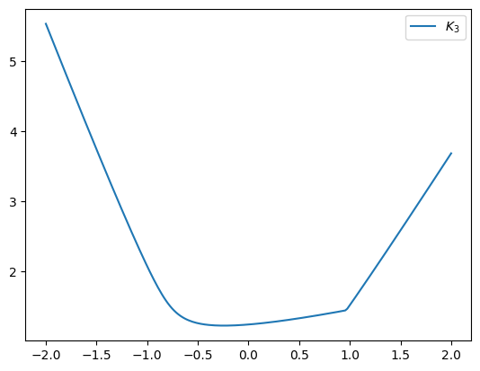
Now let’s plot the univariate function \(x \to M_r(\boldsymbol A + x \boldsymbol X)\):

np.random.seed(42)
A = np.random.randint(-1, 1, (5, 5))
B = np.random.randint(-1, 1, (5, 5))

xs = np.linspace(-2, 2, 200)
Ms = A[np.newaxis, ...] + xs[..., np.newaxis, np.newaxis] * B[np.newaxis, ...]
plt.plot(xs, kyfan(Ms, 3), label='$K_3$')
plt.legend()
plt.show()

We can see the “kink”. Now let’s implement the smooth variant - we project the eigenvalues onto the appropriate simplex to compute the projection \(\boldsymbol q^*\), and compute \(\tilde{M}_{r, \alpha}(\boldsymbol W) = \langle \boldsymbol q^*, \boldsymbol \mu\rangle - \frac{\alpha}{2} \| \boldsymbol q^* \|_2^2\):

def smooth_kyfan(Ms, r, alpha=1):
    dim = Ms.shape[-1]
    eigs = sla.eigvalsh(Ms)
    prj = project_onto_capped_simplex(eigs / alpha, r)
    return (
        np.sum(eigs * prj, axis=-1) - (alpha / 2) * np.sum(np.square(prj), axis=-1)
    )

Now we can plot the smooth function with different values of the smoothing parameters \(\alpha\):

plt.plot(xs, kyfan(Ms, 3), label='$K_3$')
plt.plot(xs, smooth_kyfan(Ms, 3, alpha=1), label='$K_{3,1}$')
plt.plot(xs, smooth_kyfan(Ms, 3, alpha=0.5), label='$K_{3,0.5}$')
plt.plot(xs, smooth_kyfan(Ms, 3, alpha=0.1), label='$K_{3,0.1}$')
plt.legend()
plt.show()

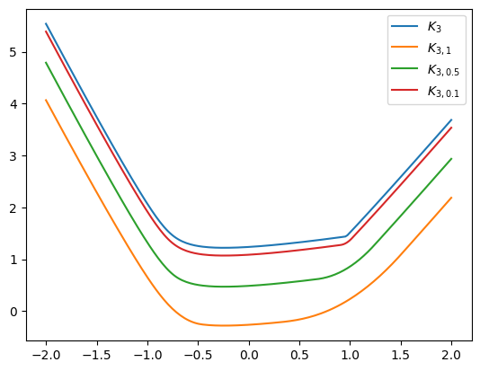
Indeed, we observe smooth functions that approach the true eigenvalue sum function \(K_3\) from below, since Moreau envelopes are smooth lower bounds.

Interestingly, we observe that the envelopes appear like shifted versions of the true function - away from the kink they share the same shape, but appear to be at a constant vertical distance. To understand why, let’s recall the projection formula - shift and clip: \(q_i^* = \operatorname{clip}(y_i + \nu, 0, 1)\) Now, if our eigenvalues are well-separated, the smaller eigenvalues will project to \(q_i^* = 0\), while the larger eigenvalues will project to \(q_i^* = 1\), so we will just obtain back the sum of the largest eigenvalues. Hence, the smoothed version and the exact version appear identical. But looking at the formula for the smoothed function:

\[\tilde{M}_{r, \alpha}(\boldsymbol W) = \langle \boldsymbol q^*, \boldsymbol \mu\rangle - \frac{\alpha}{2} \| \boldsymbol q^* \|_2^2\]

there is a \(\frac{\alpha}{2} \| \boldsymbol q^* \|_2^2\) factor that shifts us below. In case of good separation, this is just \(\frac{\alpha r}{2}\), since the projection will have \(r\) ones. This is exactly our vertical shift we see in the plot. Consequently, we can produce a better smoothed approximation in the form of \(\tilde{M}_{r, \alpha}(\boldsymbol W) + \frac{\alpha r}{2}\). Let’s visualize it:

r = 3
plt.plot(
  xs, smooth_kyfan(Ms, r, alpha=1) + 1 * r / 2,
  label='$K_{3,1} + \\frac{1 \\times 3}{2}$'
)
plt.plot(
  xs, smooth_kyfan(Ms, r, alpha=0.5) + 0.5 * r / 2,
  label='$K_{3,0.5} + \\frac{0.5 \\times 3}{2}$'
)
plt.plot(
  xs, smooth_kyfan(Ms, r, alpha=0.1) + 0.1 * r / 2, 
  label='$K_{3,0.1} + \\frac{0.1 \\times 3}{2}$'
)
plt.plot(xs, kyfan(Ms, 3), label='$K_3$', linewidth=2, alpha=0.5, linestyle='--')
plt.legend()
plt.show()

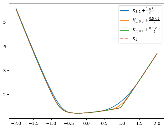
Indeed, away from the kink and the high curvature regions, the smooth approximation and the exact function align, and we’ve achieved a reasonably good smooth variant of sum-of-largest \(r\) eigenvalues with controllable gradient rate of change:

Smooth \(k\)-th smallest eigenvalue

Subtracting the two smooth approximations, we can obtain a smooth approximation of the \(k\)-th smallest eigenvalue, which is the \(r=n-k+1\)-th largest as

\[\tilde{\mu}_{r, \alpha}(\boldsymbol W) = \tilde{M}_{r, \alpha}(\boldsymbol W) - \tilde{M}_{r - 1, \alpha}(\boldsymbol W) + \frac{\alpha}{2}.\]

Here is a Python function:

def kth_eigval_smooth(Ms, k, alpha):
    n = Ms.shape[-1]
    r = n - k    # zero-based indexing
    smooth_kyfan_r_neg = smooth_kyfan(Ms, r, alpha)
    smooth_kyfan_rm1_neg = smooth_kyfan(Ms, r - 1, alpha)
    return (smooth_kyfan_r_neg - smooth_kyfan_rm1_neg + alpha / 2)

Now we can plot it, along with the exact eigenvalue:

def kth_eigval(Ms, k):
    return sla.eigvalsh(Ms, subset_by_index=(k, k))
    
plt.plot(xs, kth_eigval_smooth(Ms, 2, alpha=0.5), label='$\\lambda_{3,0.5}$')
plt.plot(xs, kth_eigval_smooth(Ms, 2, alpha=0.25), label='$\\lambda_{3,0.25}$')
plt.plot(xs, kth_eigval_smooth(Ms, 2, alpha=0.1), label='$\\lambda_{3,0.1}$')
plt.plot(xs, kth_eigval(Ms, 2), label='$\\lambda_3$', linewidth=2, alpha=0.5, linestyle='--')
plt.legend()
plt.show()

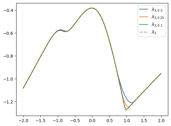
Great success! Indeed, we see a family of smooth functions that approach the true \(\lambda_3(\boldsymbol A + x \boldsymbol B)\) function.

Our kth_eigval_smooth function above computed the smooth approximation by invoking smooth_kyfan twice to compute the two smoothed top-$r$ eigenvalue sum functions. But each one of them computes the eigenvalues, and projects them onto a capped simplex. So we can compute the \(k\)-th eigenvalue directly by subtracting two projections onto the simplex:

1. Compute the non-decreasing eigenvalues \(\boldsymbol \mu(\boldsymbol W)\), and \(r=n-k+1\).
2. Compute \(\boldsymbol q_r^*\) - the projection of \(\boldsymbol \mu(\boldsymbol W) / \alpha\) onto the capped \(r\)-simplex.
3. Compute \(\boldsymbol q_{r-1}^*\) - the projection of \(\boldsymbol \mu(\boldsymbol W) / \alpha\) onto the capped \(r-1\)-simplex.
4. Output: \(\tilde{\mu}_{r, \alpha}(\boldsymbol W) = \langle \mu(\boldsymbol W), \boldsymbol q_r^* - \boldsymbol q_{r-1}^* \rangle - \frac{\alpha}{2} ( \| \boldsymbol q_r^* \|_2^2 - \| \boldsymbol q_{r-1}^* \|_2^2) + \frac{\alpha}{2}\)

Now, look at the term \(\langle \mu(\boldsymbol W), \boldsymbol q_r^* - \boldsymbol q_{r-1}^* \rangle\) - it is just a weighted sum of eigenvalues of \(\boldsymbol W\). So let’s plot these weights in the vicinity of the “kink” near \(x=1\). Here are the weights near the kink for \(\alpha = 0.5\):

alpha = 0.5
r = 3

kink_mask = (0.7 <= xs) & (xs <= 1.2)
eigs = sla.eigvalsh(Ms[kink_mask])
prj_rp1 = project_onto_capped_simplex(eigs / alpha, r)
prj_r = project_onto_capped_simplex(eigs / alpha, r - 1)
ws = prj_rp1 - prj_r

And now let’s plot these weights using a heatmap, with the \(y\)-axis being the eigenvalue index:

fig, ax = plt.subplots(figsize=(12, 6))
ax.imshow(ws.T, cmap='gray')
ax.set_xticks(
    range(sum(kink_mask)),
    labels=[f'{x:.3f}' for x in xs[kink_mask]],
    rotation=45, ha="right", rotation_mode="anchor"
)
ax.set_ylabel('$\\lambda$')
ax.set_yticks(range(Ms.shape[-1]), labels=range(1, 1 + Ms.shape[-1]))
plt.show()

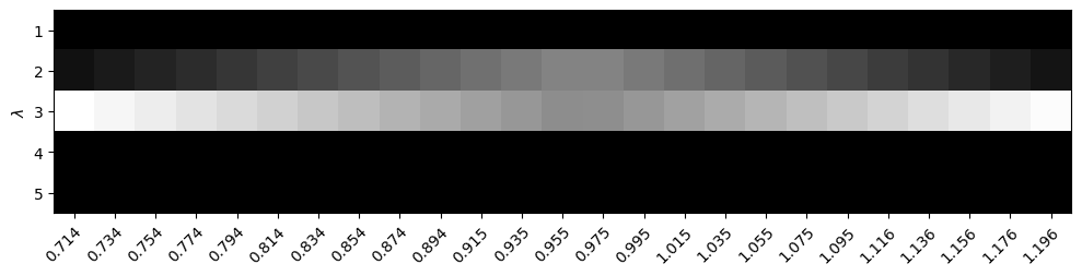
We see that we are just computing a sum of a window of two (out of five) eigenvalues. As we get closer to the “kink” there is more need for smoothing, and the weights of both eigenvalues are almost identical - we see both get a similarly gray color. But farther away from the kink, we are almost exclusively assigning all of the weight to \(\lambda_3\). The simplex projection trick automatically discovers the right weights, without us having to do the guess-work. The power of convex analysis!

So now comes the part where the math has to pay rent. The smoothing looks nice on a one-dimensional plot, but our actual goal is training. For that, the smoothed eigenvalue has to become a PyTorch operation, with a forward pass, a backward pass, and enough respect for symmetry conventions not to quietly lie to us.

The good news is that the derivation already told us what the backward pass should look like: not just one matrix \(\boldsymbol v_k \boldsymbol v_k^T\), but a weighted sum of matrices \(\boldsymbol v_j \boldsymbol v_j^T\) coming from nearby eigenvalues. The weights are exactly the capped-simplex weights we just plotted.

A smoothed eigenvalue in PyTorch

For PyTorch we will need to re-write a PyTorch variant of all our NumPy functions. Luckily, this part contains no new math - the only strange object in this post is the idea, not the syntax. We begin with almost an exact copy of the function that computes the coefficients of the piece-wise linear equation we use to project onto the simplex:

import torch

def torch_capped_simplex_coefficients(y: torch.Tensor):
    """Return breaks, intercepts, and slopes for the piecewise-linear function

        f(x) = sum_j clip(y_j - x, 0, 1).

    On each interval between two breaks,

        f(x) = intercept + slope * x.
    """
    *B, N = y.shape

    # break points and slope contribution + bias contribution at each point
    breaks = torch.cat([y - 1, y], dim=-1)
    slope_step = torch.cat([-torch.ones_like(y), torch.ones_like(y)], dim=-1)
    bias_step = torch.cat([y - 1, -y], dim=-1)

    # sort all arrays by break points
    order = torch.argsort(breaks, dim=-1)
    breaks = torch.take_along_dim(breaks, order, dim=-1)
    slope_step = torch.take_along_dim(slope_step, order, dim=-1)
    bias_step = torch.take_along_dim(bias_step, order, dim=-1)

    # create coefficients of all linear functions
    slopes = torch.cumsum(slope_step, dim=-1)
    intercepts = N + torch.cumsum(bias_step, dim=-1)

    return breaks, slopes, intercepts

Here is an analogous re-write of the equation solving function from NumPy to PyTorch:

def _torch_gather_last(a: torch.Tensor, index: torch.Tensor) -> torch.Tensor:
    return torch.take_along_dim(a, index[..., None], dim=-1)[..., 0]

def torch_solve_piecewise_linear(m, breaks, slopes, intercepts):
    value_at_breaks = intercepts + slopes * breaks

    hit_mask = value_at_breaks <= m
    hit = torch.argmax(hit_mask.to(torch.int8), dim=-1)
    seg_idx = torch.maximum(hit - 1, torch.zeros_like(hit))

    intercepts = _torch_gather_last(intercepts, seg_idx)
    slopes = _torch_gather_last(slopes, seg_idx)
    breaks = _torch_gather_last(breaks, seg_idx)

    nnz_slopes = slopes != 0
    out = breaks.detach().clone()
    out[nnz_slopes] = (m - intercepts[nnz_slopes]) / slopes[nnz_slopes]
    return out

And finally, a simple re-write of the simplex projection function:

def torch_project_onto_capped_simplex(ys, m):
    breaks, slopes, intercepts = torch_capped_simplex_coefficients(ys)
    x_sol = torch_solve_piecewise_linear(m, breaks, slopes, intercepts)
    return torch.clip(ys - x_sol[..., None], 0, 1)

Let’s see that we get similar results from NumPy and PyTorch for our vector of ys we used at the beginning of this post:

ys_torch = torch.as_tensor(ys).float()
print('NumPy: ', project_onto_capped_simplex(ys, 2))
print('Torch: ', torch_project_onto_capped_simplex(ys_torch, 2))

NumPy:  [0.   0.25 0.75 1.  ]
Torch:  tensor([0.00, 0.25, 0.75, 1.00])

Now we’re almost ready to write the autograd function. Before showing the code - there is one more simplification step. Looking at the definition of the capped \(r\)-simplex, the criteria are independent of the order of the elements. This means that if we permute the vector before projection, it is equivalent to applying the same permutation to the projection. Consequently, we don’t really need the vector of eigenvalues in nondecreasing order. It was convenient for visualization, but they can be in any order, including the order PyTorch uses.

So now we’re ready. We begin from the forward method. This is where our earlier derivation reappears almost verbatim: project the eigenvalues, divided by \(\alpha\), onto two capped simplices, subtract the projections, and use the difference as weights. When gradients are needed, we also save the eigenvectors, because the backward pass will combine the matrices \(\boldsymbol v_j \boldsymbol v_j^T\) using exactly these weights.

class KthEigvalhSmooth(torch.autograd.Function):
    @staticmethod
    def forward(ctx, Ms, k, alpha):
        need_grad = ctx.needs_input_grad[0]

        # compute just eigenvalues or also eigenvectors
        if need_grad:
            eigs, eigvecs = torch.linalg.eigh(Ms)
        else:
            eigs = torch.linalg.eigvalsh(Ms)

        # project onto capped simplices (for top n-k and top n-k-1 eigenvalues)
        n = Ms.shape[-1]
        pr = torch_project_onto_capped_simplex(eigs / alpha, n - k)
        ps = torch_project_onto_capped_simplex(eigs / alpha, n - k - 1)
        weights = pr - ps

        # save eigenvectors and weights for backward
        if need_grad:
            ctx.save_for_backward(eigvecs, weights)

        # return the difference-of-smooth-KyFan approximation + shift of alpha / 2
        return (
            (weights * eigs).sum(dim=-1)
            - 0.5 * alpha * (pr.square().sum(dim=-1) - ps.square().sum(dim=-1))
            + 0.5 * alpha
        )

Before implementing the backward pass, we need to notice something important. As a convention in PyTorch, when the symmetric eigenvalue algorithm is invoked, it uses only the lower triangle of the matrix. Why? Well - it should be symmetric, so the upper triangle is in theory just a mirror-image. In practice, it doesn’t even look at the upper triangle - it is ignored. Thus, each off-diagonal component contributes to the gradient twice: once through its role below the diagonal, and once through its mirror image above the diagonal. Diagonal components, of course, receive it only once. So below you will see a factor of two applied to off-diagonal gradients exactly because of this:

    @staticmethod
    def backward(ctx, grad_output):
        eigvecs, weights = ctx.saved_tensors

        G = (eigvecs * weights[..., None, :]) @ eigvecs.transpose(-2, -1)

        grad = torch.tril(2 * G)
        grad.diagonal(dim1=-2, dim2=-1).mul_(0.5)

        return grad_output[..., None, None] * grad, None, None

As in previous posts - here is a convenience function:

def torch_kth_eigvalh_smooth(Ms, k, tau):
    return KthEigvalhSmooth.apply(Ms, k, tau)

Now let’s verify that it works using the PyTorch torch.autograd.gradcheck function:

Ms = torch.randn(3, 5, 5)
X = torch.randn(3, 5, 5, dtype=torch.float64, requires_grad=True)

torch.autograd.gradcheck(
    lambda M: torch_kth_eigvalh_smooth(M, 2, 0.5),
    (X,),
)

True

The True means that the check has passed - the numerical gradient approximation was equivalent to our autograd implementation. This is the point where the construction stops being just a nice convex-analysis story and becomes something we can actually train with.

California housing experiments

Now comes the real test. The one-dimensional plots showed that the smoothed eigenvalue behaves the way we wanted, and gradcheck showed that our backward pass matches the numerical derivative. But the question that started this post was about training speed and stability. So let’s put the new smoothed eigenvalue model inside the same California Housing experiment we’ve been using throughout the series.

First, if we’ve already invested in being compatible with PyTorch and using only one triangle of a matrix for symmetric eigenvalue computation, let’s go all the way through and store only the lower triangle. To that end, we’ll use a small auxiliary class that reshapes a vector of \(d (d + 1) / 2\) coordinates to \(d \times d\) symmetric matrices. It’s quite simple - it precomputes the mapping from vector to matrix coordinates and stores it in a PyTorch buffer:

from torch import nn

class TrilEmbed(nn.Module):
    def __init__(self, dim: int):
        super().__init__()
        self.dim = dim

        # Get the coordinates of the lower triangle
        i, j = torch.tril_indices(dim, dim)

        # Build a lookup grid: which index of the input belongs at (row, col)?
        grid = torch.zeros(dim, dim, dtype=torch.long)
        grid[i, j] = torch.arange(len(i))

        # Symmetrize the map: copy lower indices to upper
        grid = torch.maximum(grid, grid.T)

        # Store the flattened map as a buffer
        self.map = nn.Buffer(grid.flatten())

    def forward(self, x: torch.Tensor) -> torch.Tensor:
        """
        Expands x of shape (..., K) to (..., d, d),  where K = d * (d + 1) // 2
        """
        return x[..., self.map].view(*x.shape[:-1], self.dim, self.dim)

Let’s try it out with three \(4 \times 4\) matrices:

TrilEmbed(4)(torch.randn(3, 4 * (4 + 1) // 2))

tensor([[[-0.70,  0.02, -1.30, -0.44],
         [ 0.02,  1.34, -1.52, -0.19],
         [-1.30, -1.52,  0.02, -0.35],
         [-0.44, -0.19, -0.35, -0.91]],

        [[ 0.79, -0.43,  0.53, -2.64],
         [-0.43,  0.23, -0.62, -0.71],
         [ 0.53, -0.62,  1.64,  0.42],
         [-2.64, -0.71,  0.42,  0.64]],

        [[ 1.43,  0.43, -0.56,  0.82],
         [ 0.43,  0.98, -1.37,  0.53],
         [-0.56, -1.37,  0.50, -0.42],
         [ 0.82,  0.53, -0.42, -0.33]]])

Appears to be working! Indeed, we’ve got three symmetric matrices. Now let’s write our module for

\[f(\boldsymbol x; \boldsymbol A_{0:n}) = \tilde{\lambda}_{k, \alpha}(\boldsymbol A_0 + \sum_{i=1}^n x_i \boldsymbol A_i).\]

Note, here we’re using the smoothed out version \(\tilde{\lambda}_{k, \alpha}\) we’ve just developed, rather than the exact eigenvalue. But the idea is similar - we use one neuron, composed of a linear combination of the features + a nonlinear activation in the form of the smoothed-out eigenvalue function.

Here, we shall use our module above. The linear combination is performed by an nn.Linear layer, producing \(d(d + 1) / 2\) vectors, which are then reshaped to matrices. By default, we’ll be targeting the mid-eigenvalue.

class SmoothKthEigvalhModel(nn.Module):
    def __init__(self, num_features, dim, k=None, alpha=0.1):
        super().__init__()
        self.lin = nn.Linear(num_features, dim * (dim + 1) // 2)
        self.tril_emb = TrilEmbed(dim)
        self.k = k or dim // 2
        self.alpha = alpha

    def forward(self, x):
        mat_flat = self.lin(x)
        mat = self.tril_emb(mat_flat)
        return torch_kth_eigvalh_smooth(mat, self.k, self.alpha)

As in previous posts, I will not go into the data preparation phase, and will assume that the training set is in the X_train, y_train PyTorch tensors, that the evaluation set is in the X_test, y_test tensors, that num_features contains the number of features, and that that labels y_train and y_test have been rescaled to zero mean and standard deviation of 1, and we have written the scaled_rmse function to compute root mean-squared error in the original scale.

Again, we shall use the fitstream library to simplify training:

%pip install --q fitstream
import fitstream as fts

Here is a full PyTorch training loop, implemented using fitstream, that includes a linear learning rate scheduler with \(10\%\) warmup. It produces a generator of “events” in the form of dictionaries, which we can later gather to dataframes and plot. It constructs our model, the Adam optimizer, a learning rate scheduler, and then pipes a bunch of fitstream operators. By default, we use 75 epochs, which I found to be enough for the experiments here, and a smoothing factor of \(\alpha = 0.1\), which I will use later to demonstrate an important point.

from torch.optim.lr_scheduler import OneCycleLR

def complete_training_stream(
        dim, n_epochs=75, alpha=0.1, warmup_fraction=0.1, lr=1e-2, batch_size=64,
    ):
    model = SmoothKthEigvalhModel(num_features=num_features, dim=dim, alpha=alpha)
    optim = torch.optim.Adam(model.parameters(), lr=lr)
    sched = OneCycleLR(optim, max_lr=lr, total_steps=n_epochs, pct_start=warmup_fraction, anneal_strategy='linear')

    epoch_events = fts.epoch_stream(
        (X_train, y_train), model, optim, nn.MSELoss(), batch_size=batch_size
    )
    return fts.pipe(
        epoch_events,
        fts.take(n_epochs),
        fts.augment(fts.validation_loss((X_test, y_test), scaled_rmse)),
        fts.augment(lambda event: {"lr": optim.param_groups[0]['lr']}),
        fts.tick(sched.step),
    )

Here is a short demo to show what the function yields:

for event in complete_training_stream(dim=5, n_epochs=11):
    print('step = ', event['step'], 
          ', lr = ', event['lr'], 
          ', val_loss = ', event['val_loss'])

step =  1 , lr =  0.0004 , val_loss =  90867.0078125
step =  2 , lr =  0.009090912727272728 , val_loss =  63868.4375
step =  3 , lr =  0.008080815757575757 , val_loss =  59900.1171875
step =  4 , lr =  0.007070718787878788 , val_loss =  59653.19921875
step =  5 , lr =  0.006060621818181819 , val_loss =  59391.703125
step =  6 , lr =  0.005050524848484848 , val_loss =  58910.65234375
step =  7 , lr =  0.0040404278787878785 , val_loss =  59091.203125
step =  8 , lr =  0.003030330909090909 , val_loss =  59128.265625
step =  9 , lr =  0.002020233939393939 , val_loss =  58527.10546875
step =  10 , lr =  0.0010101369696969686 , val_loss =  58274.375
step =  11 , lr =  3.999999999976245e-08 , val_loss =  58274.3671875

Indeed, we can see that we have at least the step key, which is the epoch, the lr key, which is the current learning rate, and the val_loss key, which is the validation loss. We can also see the learning rate growing the first two steps (warmup), and then decaying back (cooldown).

Recall we can also collect the stream to a dataframe, like this:

demo_log = fts.collect_pd(complete_training_stream(dim=5, n_epochs=11))

This will make plotting easier. So now we need to think what it is that we want to plot.

We began this journey from slow convergence, so somehow we need to measure not only where the model ends up, but also how it gets there. Here I propose a pretty straightforward idea - let’s measure the area under the validation loss curve. A quickly converging algorithm will tend to yield a smaller area, whereas a slowly converging one will tend to have a large area. A simple approximation is just the average of the points along the curve. Note that this incorporates both the rate, and the error we’re converging to. For example, a horizontal line, which is the fastest possible convergence, can have a terrible average if all points along the line achieve a high error.

So here is a plotting function for the validation loss from a log dataframe such as the one we produced above, together with the best validation loss we achieved, and the average of the validation loss curve:

import matplotlib.pyplot as plt

def plot_loss(log, ax_loss=None, key='val_loss', loss_label='Eval. loss', title='Loss', color='blue'):
    ax_loss = plt.gca() if ax_loss is None else ax_loss
    losses = log[key]
    ax_loss.plot(
        log.step, losses, color=color,
        label=f'{loss_label} (best={losses.min():.2f}, avg={losses.mean():.2f})'
    )
    ax_loss.set_ylabel("Loss")
    ax_loss.set_title(title)
    ax_loss.grid()
    ax_loss.legend()

It’s also informative to plot the learning rate schedule, so here it is - pretty straightforward:

def plot_lr(log, lr_ax):
    lr_ax.plot(log.step, log.lr, label='Learning rate',
               color='gray', linestyle='dotted', linewidth=1)
    lr_ax.set_ylabel("Learning rate")

And finally here is one that combines both of the above functions into one plot with two \(y\) axes - one for the loss, and one for the learning rate:

def plot_log(log, title=None):
    fig, ax_loss = plt.subplots(1, 1, figsize=(6, 4), layout='constrained')

    plot_loss(log, ax_loss, title='Error and learning rate')

    lr_ax = ax_loss.twinx()
    plot_lr(log, lr_ax)

    if title is not None:
        fig.suptitle(title)
    fig.show()

Let’s try it out:

demo_log = fts.collect_pd(complete_training_stream(dim=5, n_epochs=11))
plot_log(demo_log)

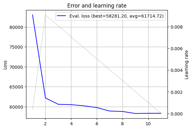
Alright! We can see the dotted line of the learning rate going up and down, and the blue line of the validation loss going down. We can also see that the best validation RMSE here is approximately \(\$58.3\)k, and that the “area under the curve” is here \(\sim \$61.7\)k.

Alright, now that we have the “piping” in place, let’s do some experiments. First, a sanity check: can the smoothed version of our neuron learn at all? Here is the result of training with \(5 \times 5\) matrices:

log_5 = fts.collect_pd(complete_training_stream(dim=5))
plot_log(log_5)

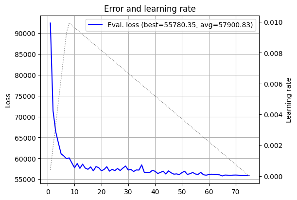
Results appear to be somewhat similar to previous posts, and it’s hard to judge much from this plot alone. But at least it is a useful sanity test: we haven’t made some embarrassing mistake - the model is learning.

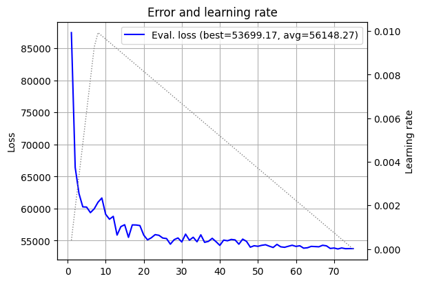
Next, let’s see whether the smoothed \(k\)-th eigenvalue still benefits from increasing the matrix size. If smoothing destroyed the useful behavior of the eigenvalue model, this is where we would start getting suspicious. Let’s try out \(7 \times 7\) matrices.

log_7 = fts.collect_pd(complete_training_stream(dim=7))
plot_log(log_7)

Nice! Both better validation loss and a smaller curve average. So the smoothing did not kill scaling, at least not yet. How about \(15 \times 15\)?

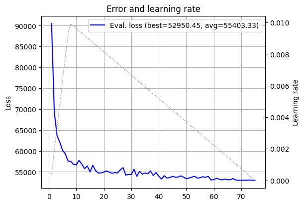
log_15 = fts.collect_pd(complete_training_stream(dim=15))
plot_log(log_15)

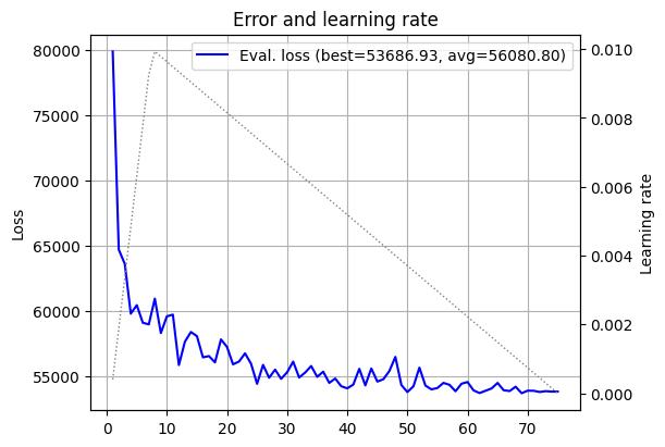
OK. Now alpha becomes the main character. Since the model becomes smoother both as a function of the features, and as a function of its parameters, a higher smoothing can help convergence, but also degrade the model’s expressive power. So there is a balance. Too little smoothing keeps us close to the original jagged eigenvalue; too much smoothing gives the optimizer an easy life, but leaves the model with less room to express interesting functions. Let’s try the same \(15 \times 15\) model, but this time with a smoothing factor of \(\alpha = 5\) (recall that the default was \(\alpha = 0.1\)).

log_15_alpha_5 = fts.collect_pd(complete_training_stream(dim=15, alpha=5))
plot_log(log_15_alpha_5)

This appears to be a better result. The best model has a lower loss, but we can also see that the loss curve flattens out earlier, and is a bit less jaggy. So far, alpha looks like a useful knob. But knobs can be turned too far. What about \(\alpha = 25\)?

log_15_alpha_25 = fts.collect_pd(complete_training_stream(dim=15, alpha=25))
plot_log(log_15_alpha_25)

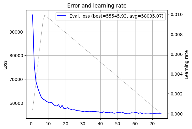
Now we see the phenomenon we discussed. The loss curve appears “nicer”, it appears to each its minimum a bit earlier, but the curve average is awful. We’ve hit the other side of the balance - our model favors the optimization process, but is not expressive enough.

Let’s also try hitting the other side of the balance with \(\alpha = 0.001\):

log_15_alpha_0_001 = fts.collect_pd(complete_training_stream(dim=15, alpha=0.001))
plot_log(log_15_alpha_0_001)

A bit hard to judge the speed, but we see that the curve average is larger than \(\alpha=5\), for example, and the loss curve itself is very jagged, almost up until the final epochs.

Let’s plot all of these curves together in one plot:

plot_loss(log_15_alpha_0_001, loss_label='$\\alpha$=0.001', color='darkblue')
plot_loss(log_15, loss_label='$\\alpha$=0.1 (default)', color='blue')
plot_loss(log_15_alpha_5, loss_label='$\\alpha$=5', color='green')
plot_loss(log_15_alpha_25, loss_label='$\\alpha$=25', color='orange')

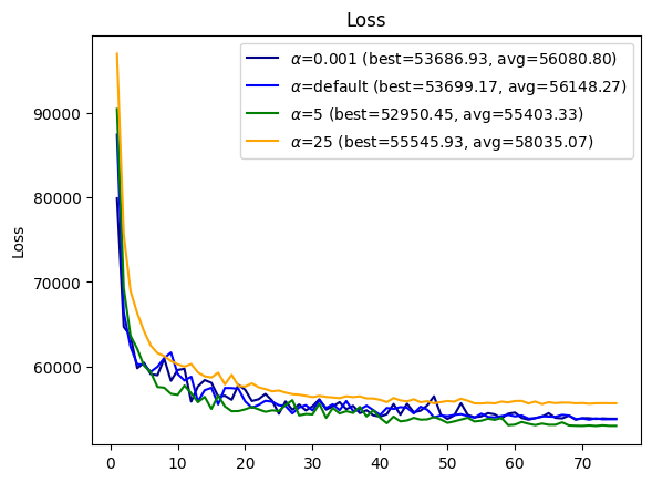
Now we can see that \(\alpha = 5\) leads - it strikes the right balance in this experiment between faster convergence and model quality. Lower \(\alpha\) values converge slower, and the larger \(\alpha=25\) value degrades model quality.

But all of this can be a matter of luck, right? Perhaps \(\alpha = 5\) got a lucky initialization, or a lucky shuffle of the data. So let’s make the comparison less anecdotal, and try several smoothing parameter values \(\alpha\) with 15 independent experiments each. Then we shall plot histograms. This experiment takes some time, \(\sim 90\) minutes in my CPU-only Colab notebook:

from tqdm.auto import tqdm

alphas = [0.001, 0.1, 5]
n_repeats = 15

records = []
for alpha in alphas:
    for _ in tqdm(range(n_repeats), desc=f'alpha = {alpha}'):
        log = fts.collect_pd(complete_training_stream(dim=15, alpha=alpha))
        auc = log['val_loss'].mean()
        records.append({'alpha': alpha, 'auc': auc})

Now that we have everything in records, let’s construct a dataframe and plot histograms using the seaborn library:

import seaborn as sns

df = pd.DataFrame.from_records(records)
g = sns.displot(df, x='auc', row='alpha', fill=False, aspect=2, height=2, hue='alpha')
g.tick_params(axis='x', rotation=45)

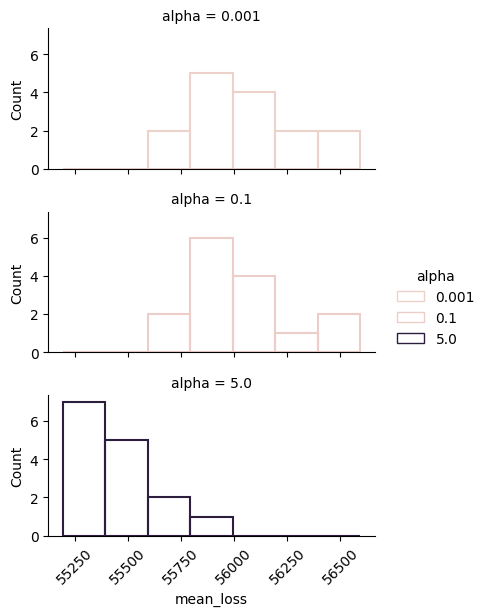
Viola! We can see indeed that \(\alpha=5\) achieves a distribution of mean loss curve values that is concentrated around smaller values, whereas smaller values of \(\alpha\), which model sharper functions, achieve higher mean loss curve values and a wider spread. In other words, training is not only slower, but also less stable.

Conclusion

In this post we tried to tackle the slow convergence problem from its root cause - colliding eigenvalues cause rapidly changing derivatives, which in turn make training slower. The Moreau-smoothed model replaces the middle eigenvalue with a carefully weighted average of a window of nearby eigenvalues. Far from a collision, almost all the weight returns to the original eigenvalue. Near a collision, the weight spreads out, and the gradient becomes much less jumpy.

But this is not magic. Smoothing the model makes a sacrifice - smoother models have less representation power. In this sense, the amount of smoothing acts as a regularizer: it makes a model more “well-behaved” while limiting what it can represent. At the same time it makes the loss more “well-behaved”, achieving faster convergence. So we need a balance between the two.

Of course, we could extend the idea to tri-diagonal matrices, or make our implementation more efficient by exploiting the fact that we need only a small window around the mid eigenvalue and thus do not require all eigenvectors for gradients. But it would make this already math-heavy post even more complex.

I think I will stop the series here. We already explored a large volume of ideas centered around eigenvalues as models. There are more ideas to explore, such as how we can scale such a model to multiple layers, or how we can build a dedicated optimizer for such models based on the convex-concave decomposition. But I think that at this stage I’d like to move to other adventures. So stay tuned!

---

References

1. Davis, C., & Kahan, W. M. (1970). The rotation of eigenvectors by a perturbation. III. SIAM Journal on Numerical Analysis, 7(1), 1-46. ↩

2. Kato, T. (2012). A short introduction to perturbation theory for linear operators. Springer Science & Business Media. ↩

3. Greenbaum, A., Li, R. C., & Overton, M. L. (2020). First-order perturbation theory for eigenvalues and eigenvectors. SIAM review, 62(2), 463-482. ↩

4. Condat, L. (2016). Fast projection onto the simplex and the l 1 ball. Mathematical Programming, 158(1), 575-585. ↩