Interpreting eigenvalue models

Intro

We continue our discussion of machine-learned models of the form

\[f({\boldsymbol x};{\boldsymbol A}_{0:n}) = \lambda_k \Bigl({\boldsymbol A}_0 + \sum_{i=1}^n x_i {\boldsymbol A}_i\Bigr),\]

where \({\boldsymbol A}_i\) are learned symmetric matrices, and \(\lambda_k\) is the \(k\)-th smallest eigenvalue. We touched on one aspect of interpretability in a previous post - the importance of each of the features \(x_1, \dots, x_n\). But there are other aspects: what does this model actually compute? How can we reason about it, or explain it to our colleagues or to a regulator? We began this series by saying that this is a “neuron” that is solving an optimization problem. So in this post we shall focus on the different kinds of optimization problems that \(f({\boldsymbol x}; {\boldsymbol A}_{0:n})\) solves, what interpretations we can give to them, and why we should care. All the results in this post are based on Chapter 4 of the Matrix Analysis book by Horn & Johnson, 2nd edition.

A game between two players

You’ve probably seen eigenvalues presented as “stretch factors”. But for our understanding of the model, the optimization view is often more useful. So here is a Courant min-max characterization of the \(k\)-th smallest eigenvalue, named after Richard Courant. It’s a bit “hairy”, so let’s first present it, and then interpret it:

\[\lambda_k({\boldsymbol A}) = \max_{ {\boldsymbol C} \in \mathbb{R}^{(k-1)\times d}} \min_{ {\boldsymbol u} \in \mathbb{R}^d} \left\{ {\boldsymbol u}^T {\boldsymbol A} {\boldsymbol u} : \| {\boldsymbol u} \|_2 = 1, \, {\boldsymbol C}{\boldsymbol u} = {\boldsymbol 0}\right\}\]

This is a bi-level optimization problem, which we can think of as a two-turn game. The first player chooses \({\boldsymbol C}\) with \(k-1\) rows (i.e., \(k-1\) linear constraints). In response, the second player chooses a unit vector \({\boldsymbol u}\) that is in the null-space of \({\boldsymbol C}\), or equivalently, orthogonal to the rows of \({\boldsymbol C}\).

The objective of the second player is to pay as little as possible, where \({\boldsymbol u}^T {\boldsymbol A} {\boldsymbol u}\) is the cost. But the objective of the first player, of course, is to make their opponent pay as much as possible, so they choose a “worst case” matrix \({\boldsymbol C}\). In case you were wondering, when \(k = 1\) we have no adversarial player, and the vector \(\boldsymbol u\) can be an arbitrary unit vector. And you have probably guessed: at any equilibrium, \({\boldsymbol u}\) is an eigenvector corresponding to \(\lambda_k({\boldsymbol A})\).

One way to read this is: \({\boldsymbol u}\) is a bounded allocation over \(d\) latent resources, and \(A_{i,j}\) is the cost associated with every pairwise interaction of resources, since:

\[{\boldsymbol u}^T {\boldsymbol A} {\boldsymbol u} = \sum_{i=1}^d \sum_{j=1}^d A_{i,j} u_i u_j\]

Depending on the context, you can give different interpretations. For example, \({\boldsymbol A}\) represents a set of latent skills a student possesses, and \({\boldsymbol u}\) is a test vector for pairs of skills.

There is a mirror-image of the above game, if we want to sort eigenvalues from largest to smallest. So the \(k\)-th largest eigenvalue, which is also the \(d-k+1\)-th smallest one, can be written as

\[\lambda_{d-k+1}({\boldsymbol A}) = \min_{ {\boldsymbol C} \in \mathbb{R}^{(k-1)\times d}} \max_{ {\boldsymbol u} \in \mathbb{R}^d} \left\{ {\boldsymbol u}^T {\boldsymbol A} {\boldsymbol u} : \| {\boldsymbol u} \|_2 = 1, \, {\boldsymbol C}{\boldsymbol u} = {\boldsymbol 0}\right\}\]

We can think of it in terms of utility rather than cost - each entry in the matrix is a utility associated with a pair of resources. The first player is choosing the matrix so that the second player will get as little utility as possible, whereas the second player, in response, aims to choose a vector \({\boldsymbol u}\) that will maximize their utility.

Adopting the \(\max-\min\) convention, we can write our “neuron” as:

\[f({\boldsymbol x};{\boldsymbol A}_{0:n}) = \max_{ {\boldsymbol C} \in \mathbb{R}^{(k-1)\times d}} \min_{ {\boldsymbol u} \in \mathbb{R}^d} \left\{ {\boldsymbol u}^T \left({\boldsymbol A}_0 + \sum_{i=1}^n x_i {\boldsymbol A}_i \right) {\boldsymbol u} : \| {\boldsymbol u} \|_2 = 1, \, {\boldsymbol C}{\boldsymbol u} = {\boldsymbol 0}\right\}\]

Consequently, each feature is associated with a matrix of some latent “costs” and our features are just the weights of these costs. Suppose you’re in the insurance business, and someone asks you what your model is doing. You can explain something like “oh, we’re representing each feature of the insured using a table of latent skills to avoid claims, we sum them up, and simulate a game where we aim to elicit their worst-case ability to either avoid damage or absorb it without claiming”. You can give an example of what those “latent skills” could be, just like in matrix factorization people explain what would be the latent features in a movie recommendation system.

As a (kind of) recurrent neural network

Another way to characterize symmetric matrix eigenvalues is as a sequence of optimization problems. Here is a Courant-Fischer formulation (Fischer here is Ernst Sigismund Fischer, not Ronald Fisher):

We just saw that the smallest eigenvalue is just the minimum of a quadratic function over the unit sphere. The second eigenvalue is similar, but the vector has to be orthogonal to one row, since the matrix \(\boldsymbol C\) the first player chooses has one row. The next eigenvalue should be orthogonal to two rows, and so on. But we can actually be more precise about what these constraints are. One of the possible formulations of the Courant-Fischer theorem is

Let \(\boldsymbol A\) be a symmetric matrix with eigenvalues \(\lambda_1 \leq \lambda_2 \leq \cdots \leq \lambda_d\) with corresponding eigenvectors \({\boldsymbol u}_1, \dots, {\boldsymbol u}_d\). Then,

\[\lambda_k = \min_{\boldsymbol u} \left\{ {\boldsymbol u}^T {\boldsymbol A} {\boldsymbol u} : \| {\boldsymbol u} \|_2 = 1,\,\langle {\boldsymbol u}, {\boldsymbol u}_1 \rangle = 0, \dots, \langle {\boldsymbol u}, {\boldsymbol u}_{k-1} \rangle = 0 \right\}\]

In other words, the \(k\)-th smallest eigenvalue is the minimum of \({\boldsymbol u}^T {\boldsymbol A} {\boldsymbol u}\) among all unit vectors orthogonal to eigenvectors corresponding to the previous eigenvalues. Thus, we can think of it as a recurrent process: computing each eigenvalue yields an eigenvector, and all eigenvectors up to \(k-1\) are used to compute the \(k\)-th eigenvalue. Visually, it looks like this:

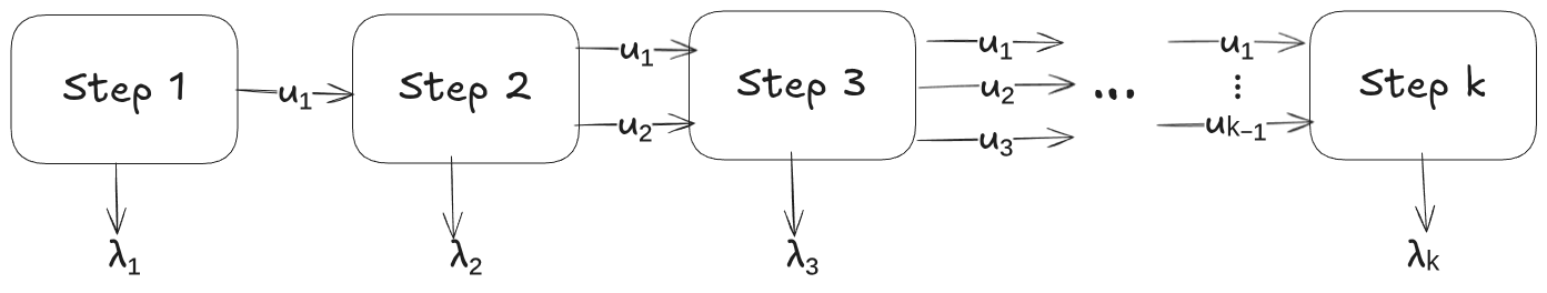
All steps share the same matrix \({\boldsymbol A}\) as their weights, just like recurrent neural networks share weights in each recurrent step.

Intuitively, as we move from \(\lambda_1\) upward, the function becomes more and more expressive. But it is tempting (and wrong) to conclude that the largest eigenvalue is the most expressive function of \({\boldsymbol A}\). Indeed, we can construct a “mirror-image” of the above process if we order the eigenvalues in decreasing order. In practice, the richest behavior tends to come from the middle of the spectrum, as we saw in the plots.

Again, we can think of this process as a kind of a repeated “game”. This time there is only one player. In each turn the player aims to minimize their cost, but their “strategy” \({\boldsymbol u}\) in each turn becomes more and more restricted - they must try something “different”, or orthogonal to, the strategies they chose in the previous turns.

As a difference of convex functions

Minimization of nonconvex functions is a long-standing challenge in optimization theory and practice. But sometimes knowing some additional information about a nonconvex function can substantially improve both the speed and the reliability of our ability to minimize it. One of these pieces of information is having an explicit representation of the function we aim to minimize (or maximize) as a difference of convex (DC) functions, namely,

\[f({\boldsymbol x}) = g({\boldsymbol x}) - h({\boldsymbol x}),\]

such that both \(g\) and \(h\) are convex. In fact, there is an entire stream of literature and algorithms on DC optimization, and many famous optimization software packages have dedicated code paths for this task. For example, the DCCP extension for CVXPY is a famous example.

Turns out our \(f({\boldsymbol x};{\boldsymbol A}_{0:n})\) has such an explicit representation and can be directly used in the DCCP extension, and other similar software packages. Why is it useful? Well, suppose \(f\) models the expected cost of some decision that we would like to minimize.

The idea is based on the Ky Fan Variational Principle, stating that the sum of the eigenvalues \(\lambda_k, \lambda_{k+1}, ..., \lambda_d\) can be written as

\[\Lambda_k({\boldsymbol A}) = \sum_{i=k}^d \lambda_i({\boldsymbol A}) = \max_{ {\boldsymbol U} \in \mathbb{R}^{(d-k+1) \times d}} \left\{ \operatorname{tr}({\boldsymbol U}^T {\boldsymbol A} {\boldsymbol U}) : {\boldsymbol U}^T {\boldsymbol U} = {\boldsymbol I} \right\}\]

This looks a bit hairy, but the term we are maximizing is a linear function of \(\boldsymbol A\), even if it’s a nonlinear function of \(\boldsymbol U\). And the maximum of linear functions is always convex, even if we have an infinite number of linear functions. Consequently, the \(k\)-th smallest eigenvalue can be written in an explicit DC form as:

\[\lambda_k({\boldsymbol A}) = \Lambda_k({\boldsymbol A}) - \Lambda_{k+1}({\boldsymbol A})\]

We can see it visually by plotting \(\lambda_k({\boldsymbol P} + x {\boldsymbol Q})\) and its two convex components as a function of \(x\):

import numpy as np
import matplotlib.pyplot as plt

# choose random matrices
np.random.seed(42)
P = np.random.randn(5, 5)
Q = np.random.randn(5, 5)

# compute eigenvalues of A + x B for x in [-3, 3]
xs = np.linspace(-3, 3, 1000)
eigvals = np.linalg.eigvalsh(P + xs[:, None, None] * Q)

# plot mid eigenvalue and its constituent convex functions
sum_top_3 = np.sum(eigvals[:, 2:], axis=-1)
sum_top_2 = np.sum(eigvals[:, 3:], axis=-1)
plt.plot(xs, sum_top_3, label=r'$\Lambda_3$')
plt.plot(xs, sum_top_2, label=r'$\Lambda_4$')
plt.plot(xs, eigvals[:, 2], label=r'$\lambda_3$')
plt.fill_between(
    xs, sum_top_3, sum_top_2,
    color='skyblue', alpha=0.2, where=(sum_top_3 > sum_top_2)
)
plt.fill_between(
    xs, sum_top_3, sum_top_2,
    color='red', alpha=0.2, where=(sum_top_3 < sum_top_2)
)
plt.grid(True, alpha=0.3)
plt.legend()

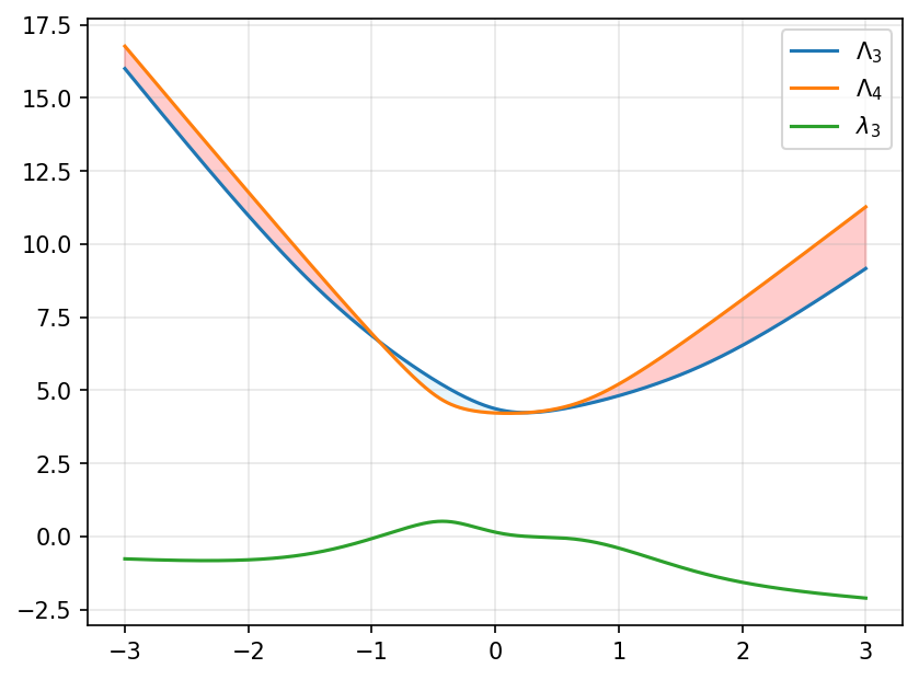
Indeed, the orange and blue plots, which are top eigenvalue sums, are convex functions. The gap between them is red when \(\Lambda_3 - \Lambda_4\) is negative, and blue when it is positive. The function in green is the difference, and it exactly reflects the size and the sign of the gap.

Recap

This was a theoretical detour, to understand what kind of functions are we fitting and how we can reason about them. We saw that we can interpret our “neuron” as a game between two players, as a recurrent process where each step solves a simple quadratic optimization problem, and as the difference between convex functions. In the next post we’re back to more practical stuff.