“Are polynomial features the root of all evil?"
This post is part of the series "Polynomial features in machine learning", and is not self-contained.
Series posts:
- “Are polynomial features the root of all evil?" (this post)
-
“Keeping the polynomial monster under control"
-
“SkLearning with Bernstein Polynomials"
-
SkLearning with Bernstein Polynomials - continued
-
A Bernstein SkLearn model calibrator
-
Regularization properties of polynomial bases
-
Let the polynomial monster free
-
Off with the polynomial's tail!
-
Paying attention to feature distribution alignment
- “Are polynomial features the root of all evil?" (this post)
- “Keeping the polynomial monster under control"
- “SkLearning with Bernstein Polynomials"
- SkLearning with Bernstein Polynomials - continued
- A Bernstein SkLearn model calibrator
- Regularization properties of polynomial bases
- Let the polynomial monster free
- Off with the polynomial's tail!
- Paying attention to feature distribution alignment
A myth
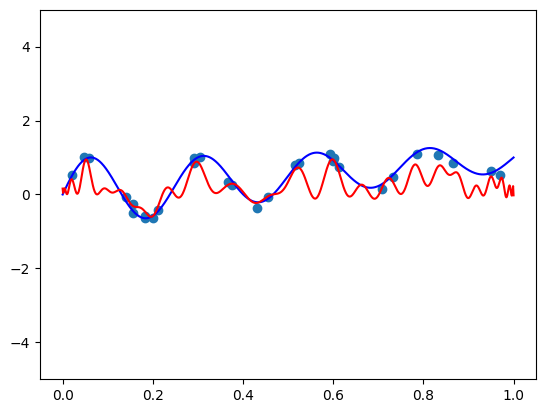
When fitting a non-linear model using linear regression, we typically generate new features using non-linear functions. We also know that any function, in theory, can be approximated by a sufficiently high degree polynomial. This result is known as Weierstrass approximation theorem. But many blogs, papers, and even books tell us that high polynomials should be avoided. They tend to oscilate and overfit, and regularization doesn’t help! They even scare us with images, such as the one below, when the polynomial fit using the data points (in red) is far away from the true function (in blue):
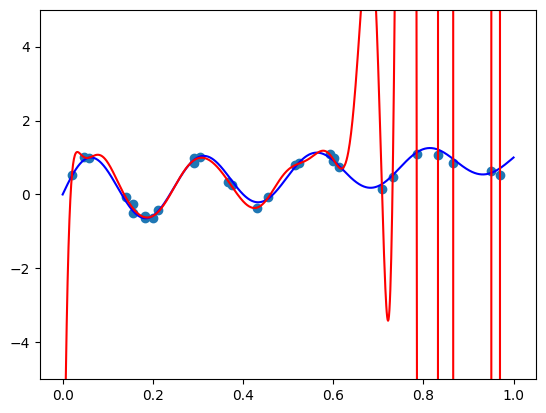
It turns out that it’s just a MYTH. There’s nothing inherently wrong with high degree polynomials, and in contrast to what is typically taught, high degree polynomials are easily controlled using standard ML tools, like regularization. The source of the myth stems mainly from two misconceptions about polynomials that we will explore here. In fact, not only they are great non-linear features, certain representations also provide us with powerful control over the shape of the function we wish to learn.
Before digging in, I want to clarify that not all properties polynomials have a notorious image for will be explored in this post. We have an entire series for that. One of those is the claim that “the biggest problem” is extrapolation. But I hope that by the end of this series you will agree with my decision to postpone it to later posts, because it is actually not “the biggest problem”. It’s actually not a problem at all.
A colab notebook with the code for reproducing the results in this post is available here.
Approximation vs estimation
Vladimir Vapnik, in his famous book “The Nature of Statistical Learning Theory” which is cited more than 100,000 times as of today, coined the approximation vs. estimation balance. The approximation power of a model is its ability to represent the “reality” we would like to learn. Typically, approximation power increases with the complexity of the model - more parameters mean more power to represent any function to arbitrary precision. Polynomials are no different - higher degree polynomials can represent functions to higher accuracy. However, more parameters make it difficult to estimate these parameters from the data.
Indeed, higher degree polynomials have a higher capacity to approximate arbitrary functions. And since they have more coefficients, these coefficients are harder to estimate from data. But how does it differ from other non-linear features, such as the well-known radial basis functions? Why do polynomials have such a bad reputation? Are they truly hard to estimate from data?
It turns out that the primary source is the standard polynomial basis for n-degree polynomials \(\mathbb{E}_n = \{1, x, x^2, ..., x^n\}\). Indeed, any degree \(n\) polynomial can be written as a linear combination of these functions:
\[\alpha_0 \cdot 1 + \alpha_1 \cdot x + \alpha_2 \cdot x^2 + \cdots + \alpha_n x^n\]But the standard basis \(\mathbb{E}_n\) is awful for estimating polynomials from data. In this post we will explore other ways to represent polynomials that are appropriate for machine learning, and are readily available in standard Python packages. We note, that one advantage of polynomials over other non-linear feature bases is that the only hyperparameter is their degree. There is no “kernel width”, like in radial basis functions1.
The second source of their bad reputation is misunderstanding of Weierstrass’ approximation theorem. It’s usually cited as “polynomials can approximate arbitrary continuous functions”. But that’s not entrely true. They can approximate arbitrary continuous functions in an interval. This means that when using polynomial features, the data must be normalized to lie in an interval. It can be done using min-max scaling, computing empirical quantiles, or passing the feature through a sigmoid. But we should avoid the use of polynomials on raw un-normalized features.
Building the basics
In this post we will demonstrate fitting the function
\[f(x)=\sin(8 \pi x) / \exp(x)+x\]on the interval \([0, 1]\) by fitting to \(m=30\) samples corrupted by Gaussian noise. The following code implements the function and generates samples:
import numpy as np

def true_func(x):
  return np.sin(8 * np.pi * x) / np.exp(x) + x

m = 30
sigma = 0.1

# generate features
np.random.seed(42)
X = np.random.rand(m)
y = true_func(X) + sigma * np.random.randn(m)
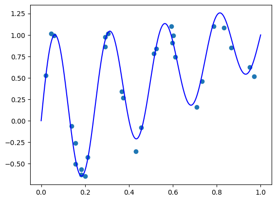
For function plotting, we will use uniformly-spaced points in \([0, 1]\). The following code plots the true function and the sample points:
import matplotlib.pyplot as plt

plt_xs = np.linspace(0, 1, 1000)
plt.scatter(X.ravel(), y.ravel())
plt.plot(plt_xs, true_func(plt_xs), 'blue')
plt.show()
Now let’s fit a polynomial to the sampled points using the standard basis. Namely, we’re given the set of noisy points \(\{ (x_i, y_i) \}_{i=1}^m\), and we need to find the coefficients \(\alpha_0, \dots, \alpha_n\) that minimize:
\[\sum_{i=1}^m (\alpha_0 + \alpha_1 x_i + \dots + \alpha_n x_i^n - y_i)^2\]As expected, this is readily accomplished by transforming each sample \(x_i\) to a vector of features \(1, x_i, \dots, x_i^n\), and fitting a linear regression model to the resulting features. Fortunately, NumPy has the numpy.polynomial.polynomial.polyvanderfunction. It takes a vector containing \(x_1, \dots, x_m\) and produces the matrix
The name of the function comes from the name of the matrix - the Vandermonde matrix. Let’s use it to fit a polynomial of degree \(n=50\). Yes, a degree higher than the number of points. There is a reason - I promised you we’ll learn not to feat high degree polynomials :)
from sklearn.linear_model import LinearRegression
import numpy.polynomial.polynomial as poly

n = 50
model = LinearRegression(fit_intercept=False)
model.fit(poly.polyvander(X, deg=n), y)
The reason we use fit_intercept=False is because the ‘intercept’ is provided by the first column of the Vandermonde matrix. Now we can plot the function we just fit:
plt.scatter(X.ravel(), y.ravel())                                    # plot the samples
plt.plot(plt_xs, true_func(plt_xs), 'blue')                          # plot the true function
plt.plot(plt_xs, model.predict(poly.polyvander(plt_xs, deg=n)), 'r') # plot the fit model
plt.ylim([-5, 5])
plt.show()
As expected, we got the “scary” image from the beginning of this post. Indeed, the standard basis is awful for model fitting! We hope that regularization provides a remedy, but it does not. Maybe adding some L2 regularization helps? Let’s use the Ridge class from the sklearn.linear_model package to fit an L2 regularized model:
from sklearn.linear_model import Ridge

reg_coef = 1e-7
model = Ridge(fit_intercept=False, alpha=reg_coef)
model.fit(poly.polyvander(X, deg=n), y)

plt.scatter(X.ravel(), y.ravel())                                    # plot the samples
plt.plot(plt_xs, true_func(plt_xs), 'blue')                          # plot the true function
plt.plot(plt_xs, model.predict(poly.polyvander(plt_xs, deg=n)), 'r') # plot the fit model
plt.ylim([-5, 5])
plt.show()
We get the following result:
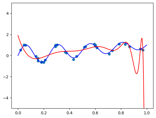
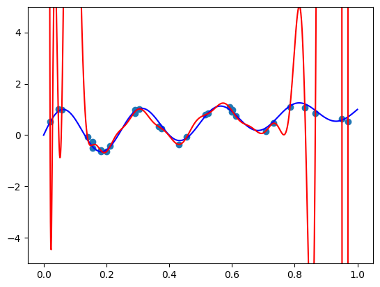
The regularization coefficient coefficient of \(\alpha=10^{-7}\) is large enough to excessively smooth out the model in \([0,0.8]\) but not large enough to avoid large oscilations in \([0.8, 1]\). Increasing the coefficient clearly won’t help - the model will be overly smoothed even further in \([0, 0.8]\).
Since we will be trying several polynomial bases, it makes sense to write a more generic function for our experiments that will accept various “Vandermonde” matrix functions of the basis of our choice, fit the polynomial using the Ridge class, and plot it with the original function and the sample points.
def fit_and_plot(vander, n, alpha):
  model = Ridge(fit_intercept=False, alpha=alpha)
  model.fit(vander(X, deg=n), y)

  plt.scatter(X.ravel(), y.ravel())                           # plot the samples
  plt.plot(plt_xs, true_func(plt_xs), 'blue')                 # plot the true function
  plt.plot(plt_xs, model.predict(vander(plt_xs, deg=n)), 'r') # plot the fit model
  plt.ylim([-5, 5])
  plt.show()
Now we can reproduce our latest experiment by invoking:
fit_and_plot(poly.polyvander, n=50, alpha=1e-7)
Polynomial bases
It turns out that in our sister discipline, approximation theory, reseachers also encountered similar difficulties with the standard basis \(\mathbb{E}_n\), and developed a thoery for approximating functions by polynomials from different bases. Two prominent examples of bases of \(n\)-degree polynomials include, and their:
- The Chebyshev polynomials \(\mathbb{T}_n = \{ T_0, T_1, \dots, T_n \}\), implemented in the
numpy.polynomial.chebyshevmodule. - The Legendre polynomials \(\mathbb{P}_n = \{ P_0, P_1, \dots, P_n \}\), implemented in the
numpy.polynomial.legendremodule.
They are the computational workhorse of a large variety of numerical algorithms that are enabled by approximating a function using a polynomial, and are well-known for their advantages in approximating functions in the \([-1, 1]\) interval2. In particular, the corresponding “Vandermonde” matrices are provided by the chebvander and legvander functions in corresponding modules above. Each row in these matrices contains the value of the basis functions at each point, just like the standard Vandermonde matrix of the standard basis. For example, the Chebyshev Vandermonde matrix is:
I will not elaborate their formulas and properties here for a reason that will immediately be revealed. However, I highly recomment Prof. Nick Trefethen’s “Approximation theory and approximation practice” online video course to get familiar with their advantages. His book with the same name is an excellent introduction to the subject.
It might be tempting to try fitting a Chebyshev polynomial using our fit_and_plot method above directly:
import numpy.polynomial.chebyshev as cheb

fit_and_plot(cheb.chebvander, n=50, alpha=1e-7)
However, that’s not the best thing to do. We aim to fit a function sampled from \([0, 1]\), but the Chebyshev basis “lives” in \([-1, 1]\). Therefore, we will add the transformation \(x \to 2x-1\) before invoking the chebvander function:
def scaled_chebvander(x, deg):
  return cheb.chebvander(2 * x - 1, deg=deg)

fit_and_plot(scaled_chebvander, n=50, alpha=1)
Note that a different basis requires a different regularization coefficient. We get the following result:
Whoa! Seems even worse than the standard basis!. Maybe more regularization helps?
fit_and_plot(scaled_chebvander, n=50, alpha=10)
Appears that our polynomial is both a bad fit for the function, and extremely oscilatory. Even worse when the standard basis! Interested readers can repeat the experiment with Legendre polynomials and see a slightly better, but similar result. You can also try making it of degree 29, so that the number of parameters is equal to the number of samples, and get even worse results! So what’s wrong? Well, we will explore these two later in this series, but at this stage we’ll say they are useful for the fitting problem in two cases - when the degree is either much smaller or much larger than the number of samples. And no, the much larger is not a typo. This small experiment is here to demonstrate that results from approximation theory not always directly transfer to results in machine learning. The task of fitting differs form the task of approximation.
So let’s introduce another interesting basis that we shall explore here and in the following posts, since it turns out to be extremely useful for various fitting tasks.
The Bernstein basis
The Bernstein basis \(\mathbb{B}_n = \{ b_{0,n}, \dots, b_{n, n} \}\) are \(n\)-degree polynomials defined by on \([0, 1]\) by:
\[b_{i,n}(x) = \binom{n}{i} x^i (1-x)^{n-i}\]These polynomials are widely used in computer graphics to approximate curves and surfaces, but it appears that they’re less known in the machine learning community. In fact, all the text you see on the screen when reading this post is rendered using Bernstein polynomials3. We will study them more in depth in the next posts, but at this stage I would like to point out two simple properties that give an intuitive explanation of why they’re useful in machine learning.
First, note that each \(b_{i,n}\) is an \(n\)-degree polynomial. Thus, when representing a polynomial using
\[p_n(x) = \alpha_0 b_{0,n}(x) + \alpha_1 b_{1,n}(x) + \dots + \alpha_n b_{n,n}(x),\]all the coefficients have the same “units”.
If the formula of \(b_{i,n}(x)\) seems familiar - you are correct. It is exactly the probability mass function of the binomial distribution for obtaining \(i\) successes in a sequence of trials whose success probability is \(x\). Therefore, \(b_{i,n}(x) \geq 0\), and \(\sum_{i=0}^n b_{i,n}(x) = 1\) for any \(x \in [0, 1]\). Consequently, the polynomial \(p_n(x)\) is just a weighted average of the coefficients \(\alpha_0, \dots, \alpha_n\). So not only the coefficients have the same “units”, their “units” are also the same as the model’s outputs. Thus, they’re much easier to regularize - they’re all on the same “scale”.
Finally, due to the equivalence with the binomial distribution p.m.f, we can implement a “Vandermonde” matrix in Python using the scipy.stats.binom.pmf function.
from scipy.stats import binom

def bernvander(x, deg):
	return binom.pmf(np.arange(1 + deg), deg, x.reshape(-1, 1))
Let’s try and fit without regularization at all
fit_and_plot(bernvander, n=50, alpha=0)
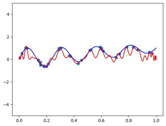
We see our regular over-fitting. Now let’s see that they’re indeed easy to regularize. After trying several regularization coefficients, I came up with this:
fit_and_plot(bernvander, n=50, alpha=5e-7)
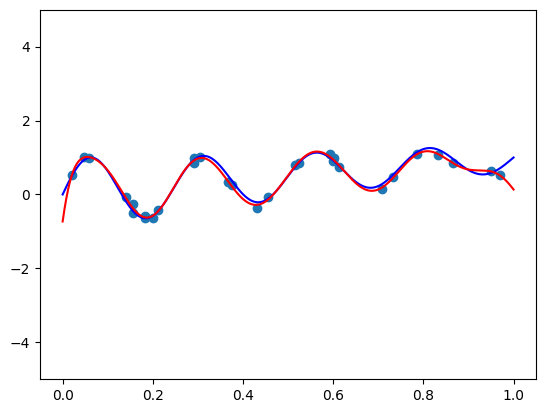
Beautiful! This is a polynomial of degree 50! The fit is great, no oscillations, and the misfit near the right endpoint stems from the noise - I don’t believe there’s enough information in the data to convey the fact that it should “curve up” rather than “curve down”.
Let’s see what happens when we crank-up the degree. Can we produce a nice non-oscilating polynomial?
fit_and_plot(bernvander, n=100, alpha=5e-4)
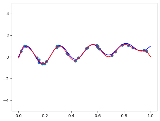
This is a polynomial of degree 100, that does not overfit!
Are we cheating?
One last message I want to convey before we wrap up is that our nice results are not cheating. You can in theory work with \([-100, 100]\) and use the basis
\[\hat{b}_{i,n}(x) = b_{i,n}(\tfrac{x}{200} + 0.5),\]which is just Bernstein polynomials applied to normalized features. Why isn’t it cheating? Because \(\hat{b}_{i,n}(x)\) is also a polynomial! Nobody forces to compute this polynomial by raising large magnitude numbers to high degrees. The way mathematical objects are defined and the way they are employed computationally can, and oftentimes should differ.
In fact, this is very common in machine learning! For example, consider the cross-entropy loss. Many of us train multi-class classifiers, and even all our LLMs are pre-trained with it! But at its core is the function
\[\operatorname{LogSumExp}(\mathbf{x}) = \ln\left( \sum_i e^{x_i} \right).\]Whoa! Exponentials! They overflow easily! But for some reason statistics and ML textbooks are not trying to convince you not to use it. The contrary - they encourage it! Why? Because our ML packages know how to compute it in a numerically stable manner that is not by definition. The same with polynomials - we compute with polynomials not by definition, but by using carefully designed algorithms.
Summary
The notorious reputation of high-degree polynomials in the machine learning community is primarily a myth. Despite it, papers, books, and blog posts are based on this premise as if it was an axiom. Bernstein polynomials are little known in the machine learning community, but there are a few papers45 using them to represent polynomial features. Their main advantage is ease of use - we can use high degree polynomials to exploit their approximation power, and ease of regularization with the right basis.
I hope the post convinced you that high degree polynomials may be useful, and you want to discover more in this series. I hope the message that the main issue is the standard basis, and not the fact that we’re working in \([0, 1]\) or any other “cheating” has been conveyed. Even in \([0, 1]\), we weren’t able to get a good fit with the standard basisl!
In the following posts we will explore the Bernstein basis in more detail. We will use it to create polynomial features for real-world datasets and test it versus the standard basis. Moreover, we will see how to regularize the coefficients to control the shape of the function we aim to represent.. For example, what if we know that the function we’re aiming to fit is increasing? Stay tuned!
-
There are also kernel methods, and polynomial kernels. But polynomial kernels suffer from problems similar to the standard basis. ↩
-
The standard basis is not that awful. It’s a great basis for representing polynomials on the complex unit circle. In fact, the Fourier transform is based exactly on this observation. ↩
-
See Bézier curves and TrueType font outlines. ↩
-
Marco, Ana, and José-Javier Martı. “Polynomial least squares fitting in the Bernstein basis.” Linear Algebra and its Applications 433.7 (2010): 1254-1264. ↩
-
Wang, Jiangdian, and Sujit K. Ghosh. “Shape restricted nonparametric regression with Bernstein polynomials.” Computational Statistics & Data Analysis 56.9 (2012): 2729-2741. ↩