Intro

Efficiency is a quiet superpower in research. When training is fast, you can iterate: try an idea, get surprised, debug, tune, and move on. When training is slow, you start avoiding experiments you should be running, simply because they cost too much time.

This became very tangible in this eigenvalue-model series. In the previous posts we looked at models that predict the $k$-th eigenvalue of a learned symmetric matrix built from the input features, and we explored what they can represent, plus some robustness/interpretability properties. Naturally, the next step was to scale up the matrix size and see what happens in practice.

I did not show it in the last post, but if you take the California Housing experiment and run $30\times 30$ matrices for 500 epochs, it takes more than an hour on Colab. And this is with an L4 GPU. I even tried an A100, and it didn’t meaningfully improve anything. So then I asked myself - what’s wrong?

Turns out PyTorch is wrong. torch.linalg.eigvalsh has a note in the official documentation: when the input is on CUDA, it synchronizes the device with the CPU. If eigenvalues sit inside your inner training loop, that synchronization becomes the bottleneck, and the rest of your model almost doesn’t matter.

So this post is a practical detour: we’ll make eigenvalue computation fast enough that it stops getting in the way. We’ll replace the slow call with a faster GPU implementation, and we’ll wrap it in a way that still supports backprop through the $k$-th eigenvalue. Once that’s done, the scaling experiments from the previous post become feasible again, and we can go back to asking the interesting questions.

(All execution speeds I measure in this post are on Colab, with an NVIDIA L4 GPU, with the 2025.10 runtime.)

Warm-up

Let’s start from a simple eigenvalue computation test on the CPU. We’ll use Jupyter’s %%time magic keyword to measure time. First, let’s create a mini-batch of 500 matrices of size 100x100:

mats = torch.randn(500, 100, 100)

Now let’s see how fast we can compute the sum of eigenvalues of all these matrices:

%%time
torch.linalg.eigvalsh(mats).sum()

CPU times: user 223 ms, sys: 14.4 ms, total: 237 ms
Wall time: 188 ms
tensor(56.6666)

And now with NumPy:

import numpy as np

# in another cell
%%time
np.linalg.eigvalsh(mats.numpy()).sum()

CPU times: user 942 ms, sys: 7.07 ms, total: 949 ms
Wall time: 337 ms

np.float32(56.665924)

Apparently, on the CPU, NumPy is almost twice slower than PyTorch. So when our tensors are on the CPU, we can continue using PyTorch - it’s pretty fast.

Now let’s move to the GPU. Here is a similar piece of code - create a mini-batch of random matrices and compute the sum of their eigenvalues:

mats = torch.randn(500, 100, 100, device='cuda')
torch.linalg.eigvalsh(mats).sum()

The reason I ran the eigenvalue computation once is as a “warmup” - I want PyTorch to do whatever setup it needs to run CUDA kernels, so next time we invoke eigvalsh it is going to be a “clean” run not contaminated by setup:

%%time
torch.linalg.eigvalsh(mats).sum()

CPU times: user 788 ms, sys: 811 µs, total: 789 ms
Wall time: 788 ms
tensor(-557.2836, device='cuda:0')

Whoa! It’s twice slower than NumPy on CPU, and four times slower than PyTorch on the CPU! Turns out PyTorch developers haven’t invested that much in general-purpose scientific computing on the GPU. It’s quite reasonable - it is not their main focus. So if we want to propose a new computational tool - it’s up to us to make it efficient!

So maybe PyTorch hasn’t invested in eigenvalues on GPU that much, but it doesn’t mean other scientific computing libraries haven’t. CuPy, a library aiming to be “NumPy on CUDA”, is one of those libraries that has a very fast eigenvalue solver we can use. But how can we use it on PyTorch tensors?

Turns out there is a standard called DLPack for representing multi-dimensional tensors in memory, and it is supported both by PyTorch and by CuPy. In PyTorch we have the torch.utils.dlpack package for converting a tensor to a DLPack “capsule” - a wrapper around its memory with appropriate metadata:

from torch.utils import dlpack as torch_dlpack

x = torch.tensor([1, -2, 3], device='cuda')
torch_dlpack.to_dlpack(x)

<capsule object "dltensor" at 0x7b9a1ae26760>

We can use CuPy to consume this “capsule” and access the same tensor, but this time as a CuPy array:

import cupy as cp

cp.from_dlpack(torch_dlpack.to_dlpack(x))

array([ 1, -2,  3])

Now let’s try computing the sum of eigenvalues of our PyTorch mats tensor containing the mini-batch of matrices using CuPy:

cupy_mats = cp.from_dlpack(torch_dlpack.to_dlpack(mats))
cp.linalg.eigvalsh(cupy_mats).sum()

array(-557.284, dtype=float32)

We got the same value, so apparently it’s working. Let’s time it:

%%time
cp.linalg.eigvalsh(cupy_mats).sum()

CPU times: user 1.58 ms, sys: 0 ns, total: 1.58 ms
Wall time: 1.37 ms
array(-557.284, dtype=float32)

Now that’s FAST! 1.37 milliseconds, instead of more than 700 - almost 500 times faster! It’s impressive, but a part of the enormous speedup is because we aren’t doing anything to be prepared to backpropagate.

Of course we got a CuPy array of eigenvalues. But we can easily use DLPack to convert it back to a PyTorch tensor. Since there is no memory copy, it practically incurs no cost, as you can see below:

%%time
eigvals_cupy = cp.linalg.eigvalsh(cupy_mats)
torch_dlpack.from_dlpack(eigvals_cupy).sum()

CPU times: user 1.66 ms, sys: 0 ns, total: 1.66 ms
Wall time: 1.31 ms
tensor(-557.2838, device='cuda:0')

Here, the eigenvalues were computed with CuPy, but their sum was computed with PyTorch. You can see that we got the same result at the same speed, since DLPack conversions just wrap the same GPU memory block, without any copies.

So the process is simple:

Wrap our PyTorch tensor’s memory as a CuPy array via DLPack
Compute eigenvalues using CuPy
Convert eigenvalues back to PyTorch via DLPack

There are more nuances here about memory management, and which object is responsible for actually freeing the memory when it’s no longer needed, and you should learn these DLPack nuances if you wish to use it. But that’s out of the scope of this post.

What we have is still not enough to build a full-fledged function we can use for model training in PyTorch, since for training we also need gradients.

Eigenvalue gradients

Consider the function

\[f({\boldsymbol X}) = \lambda_k({\boldsymbol X})\]

of a symmetric matrix $\boldsymbol X$. Recall from linear algebra that eigenvalues are roots of polynomials, and polynomial roots can have multiplicities - the same root can “repeat” multiple times.

For simplicity, assume for now that at our point of interest we have a simple eigenvalue, namely, with multiplicity 1. In this case, a well-known result from linear algebra is that it has a unique (up to sign) normalized eigenvector ${\boldsymbol q}_k({\boldsymbol X})$. Turns out that the function $f$ is differentiable at such points, and the gradient is simple:

\[\nabla f({\boldsymbol X}) = {\boldsymbol q}_k({\boldsymbol X}) {\boldsymbol q}_k({\boldsymbol X})^T.\]

Thus, the only thing we need for back-propagation is the eigenvector corresponding to our desired eigenvalue - its outer product with itself is the gradient.

Let’s convince ourselves that this works with code. Here is the outer product of the eigenvector corresponding to the middle eigenvalue of a $5 \times 5$ matrix with itself:

mat = torch.linspace(-5, 5, 25).reshape(5, 5)
w, Q = torch.linalg.eigh(mat)
i = 2
grad_mat = Q[:, i].view(-1, 1) @ Q[:, i].view(1, -1)
grad_mat

tensor([[ 0.1389, -0.2269, -0.0168,  0.2359, -0.1102],
        [-0.2269,  0.3708,  0.0274, -0.3855,  0.1801],
        [-0.0168,  0.0274,  0.0020, -0.0285,  0.0133],
        [ 0.2359, -0.3855, -0.0285,  0.4008, -0.1873],
        [-0.1102,  0.1801,  0.0133, -0.1873,  0.0875]])

And here is the gradient computed by taking the mid eigenvalue and applying tensor.backward() to compute the gradient:

mat_param = torch.nn.Parameter(torch.linspace(-5, 5, 25).reshape(5, 5))
w = torch.linalg.eigvalsh(mat_param)
w[i].backward()
mat_param.grad

tensor([[ 0.1389, -0.2269, -0.0168,  0.2359, -0.1102],
        [-0.2269,  0.3708,  0.0274, -0.3855,  0.1801],
        [-0.0168,  0.0274,  0.0020, -0.0285,  0.0133],
        [ 0.2359, -0.3855, -0.0285,  0.4008, -0.1873],
        [-0.1102,  0.1801,  0.0133, -0.1873,  0.0875]])

Things become more complicated when the eigenvalue is not simple, and has a multiplicity of at least two. In this case the function is not differentiable, and this is exactly the cause of the “kinks” we saw in the first post in the series, where we aimed to understand what kind of functions are representable using our “eigenvalue neuron”.

There are many notions of “generalized derivatives”, and we will have to choose one that is appropriate. Now here is a spoiler alert - we can still take one of the eigenvectors, call it ${\boldsymbol q}_k$, and use the vector ${\boldsymbol q}_k {\boldsymbol q}_k^T$ for back-propagation. So now that we know what code to write, let’s try to understand why.

Consider the well-known ReLU function with a kink at zero. To the left of zero, the derivative is zero. To the right of zero, it is one. At zero there is no derivative, but we can use any number between zero and one. Intuitively, we understand it’s because any line with a slope between zero and one can behave like a tangent - it touches the function at one point. Now note one important point - I said any number between zero and one. So we don’t have one slope we can use - we have an infinity of them.

A generalization of this idea of using the set of vectors “in between neighboring gradients” is known as the Clarke sub-differential¹. In higher dimensions, “in-between” generalizes to the closure of the convex hull. I am not going deep into theory, so we’ll not discuss exactly the convex hull of what we are taking, but intuitively these are gradients in a small neighborhood. If you’re interested, I have a great book² by Frank Clarke himself to recommend :)

Clarke sub-differential is one of these notions of generalized derivatives that are typically accepted as the “right” one for back-prop ³⁴. We are not always guaranteed to get an element in the Clarke sub-differential⁴ when backpropagating through a large graph, but we should do our best at least for our atomic building blocks. And just like we can take any slope between 0 and 1 for ReLU, we can take any vector in sub-differential set. Turns out our outer product of an eigenvector with itself is an element of the Clarke sub-differential set for the $k$-th eigenvalue function.

Now we have our two ingredients - a way to quickly compute eigenvalues and eigenvectors on the GPU, and a way to compute the gradient for backpropagation - so let’s finally create our PyTorch function!

A custom $k$-th eigenvalue function

First, we’ll need two utilities to convert tensors from PyTorch to CuPy and back via DLPack:

def _torch_to_cupy(x: torch.Tensor):
    """ Zero-copy via DLPack for CUDA """
    return cp.from_dlpack(torch_dlpack.to_dlpack(x))

def _cupy_to_torch(x_cupy):
    """ Zero-copy via DLPack for CUDA """
    return torch_dlpack.from_dlpack(x_cupy)

Implementing a custom PyTorch autograd function is quite simple - we just need to follow a template. We inherit from torch.autograd.Function and implement two static methods - forward and backward. The former computes our function, and optionally caches anything required for computing the derivative. The latter just back-propagates the derivative. Moreover, to make things efficient, typically forward is split into two code paths - one efficient path when no derivatives are required (inference mode), and another one for the case when derivatives are required. So here it is:

class CuPyKthEigval(torch.autograd.Function):
    @staticmethod
    def forward(ctx, A: torch.Tensor, k: int, lower: bool = True):
        # A: PyTorch --> CuPy
        A_ = A if A.is_contiguous() else A.contiguous()
        A_cp = _torch_to_cupy(A_.detach())

        # Which part of A to use, in CuPy language
        uplo = "L" if lower else "U"

        if ctx.needs_input_grad[0]: # for training
            # CuPy eigenvalues and eigenvectors
            ws_cp, Qs_cp = cp.linalg.eigh(A_cp, UPLO=uplo)
            
            # CuPy --> PyTorch
            ws = _cupy_to_torch(ws_cp).to(dtype=A.dtype, device=A.device)
            Qs = _cupy_to_torch(Qs_cp).to(dtype=A.dtype, device=A.device)
            
            # Store k-th eigenvector for the derivative
            ctx.save_for_backward(Qs[..., k].unsqueeze(-1))
        else: # for inference
            ws_cp = cp.linalg.eigvalsh(A_cp, UPLO=uplo)
            ws = _cupy_to_torch(ws_cp).to(dtype=A.dtype, device=A.device)

        return ws[..., k] # k-th eigenvalue

    @staticmethod
    def backward(ctx, grad_w: torch.Tensor):
        (Q,) = ctx.saved_tensors  # (..., n, 1)
        grad_w = grad_w.to(dtype=Q.dtype)
        grad_A = (Q * grad_w[..., None, None]) @ Q.transpose(-1, -2)
        return grad_A, None, None  # no grad for `k` and `lower`

It’s a bit lengthy, but straightforward. We just follow the sketch we laid about above. To use our new function, we just need to call the apply function of our new class:

mat_param = torch.nn.Parameter(torch.linspace(-5, 5, 25, device='cuda').reshape(5, 5))
w = CuPyKthEigval.apply(mat_param, 2)
w.backward()
mat_param.grad

tensor([[ 0.1389, -0.2269, -0.0168,  0.2359, -0.1102],
        [-0.2269,  0.3708,  0.0274, -0.3855,  0.1801],
        [-0.0168,  0.0274,  0.0020, -0.0285,  0.0133],
        [ 0.2359, -0.3855, -0.0285,  0.4008, -0.1873],
        [-0.1102,  0.1801,  0.0133, -0.1873,  0.0875]], device='cuda:0')

Identical to the gradient we previously obtained - so as a sanity check, this appears to be working. Now let’s measure the speed versus PyTorch with a mini-batch of 500 matrices of size $50 \times 50$:

mats = torch.randn(500, 100, 100, device='cuda')
mat_param = torch.nn.Parameter(torch.randn(500, 100, 100, device='cuda'))

%%time 
w = CuPyKthEigval.apply(mats, 2).sum()

CPU times: user 1.44 ms, sys: 993 µs, total: 2.43 ms
Wall time: 2.1 ms

Alright, 2 milliseconds. Pretty fast. What happens if we need backpropagation?

%%time
w = CuPyKthEigval.apply(mat_param, 2).sum()
w.backward()

CPU times: user 81.3 ms, sys: 1 µs, total: 81.3 ms
Wall time: 81 ms

Much slower! But we also understand why - we need the eigenvector, not just the eigenvalue. What about PyTorch?

CPU times: user 795 ms, sys: 0 ns, total: 795 ms
Wall time: 794 ms

Apparently, our custom function, even with backprop, is almost 10 times faster! Things appear much better, and we can move forward. As a final step, we now wrap it with a convenience function to separate the CUDA tensors from non-CUDA tensors:

def faster_kth_eigvalh(
        A: torch.Tensor, k: int,  *, lower: bool = True
    ) -> torch.Tensor:
    if A.is_cuda:
        return CuPyKthEigval.apply(A, k, lower)
    else:
        return torch.linalg.eigvalsh(A, lower)[..., k]

Nice! So now we have a function that works quickly on a GPU and we can finally do an experiment that I was not able to do in the previous post within a reasonable amount of time - try even larger matrices!

Trying it out in practice

Recall that in the last post we implemented a class, called MultivariateSpectral, for the model family we study in this series:

\[f(\mathbf{x}; {\boldsymbol \mu}, \mathbf{A}_{1:n}) = \lambda_k \left( \operatorname{diag}({\boldsymbol \mu}) + \sum_{i=1}^n x_i \mathbf{A}_i \right),\]

where the non-decreasing vector ${\boldsymbol \mu}$ and the symmetric matrices $\mathbf{A}_1, \dots, \mathbf{A}_n$ are the learned parameters. Here is a version of it that uses our new faster_kth_eigvalh function:

class MultivariateSpectral(nn.Module):
    def __init__(self, *, num_features: int, dim: int, eigval_idx: int):
        super().__init__()
        self.eigval_idx = eigval_idx
        self.mu = Nondecreasing(dim) # <-- we wrote it in the last post
        self.A = nn.Parameter(
            torch.randn(num_features, dim, dim) / (math.sqrt(dim) * num_features)
        )

    def forward(self, x):
        # batches of sum of x[i] * A[i]
        nf, dim = self.A.shape[:2]
        feature_mat = (x @ self.A.view(nf, dim * dim)).view(-1, dim, dim)

        # diag(mu) replicated per batch
        bias_mat = torch.diagflat(self.mu()).expand_as(feature_mat)

        # batched eigenvalue computation
        return self._compute_eigval(bias_mat + feature_mat)

    def _compute_eigval(self, mat):
        return faster_kth_eigvalh(mat, self.eigval_idx)

To be able to test it against PyTorch, here is a variant that uses the regular PyTorch eigenvalue function - we just inherit the above class and override the _compute_eigval function:

class MultivariateSpectralTorch(MultivariateSpectral):
    def _compute_eigval(self, mat):
        return torch.linalg.eigvalsh(mat)[..., self.eigval_idx]

So now we will use functions we implemented in the last post to again test ourselves on supervised regression with the California Housing dataset.

In the last post we implemented the function train_model_stream that trains the given model and yields a sequence of dictionaries containing the model and the training loss, and the add_spectral_norms which augments this dictionary with spectral norms of the learned matrices that we used for obtaining a global bound on the model’s sensitivity with respect to features. Here we shall just use these helpers assuming they are defined, and that the dataset is already loaded and pre-processed. The linked notebook at the beginning of this post contains the full code.

So let’s measure how long 5 training epochs take with PyTorch eigenvalues. Again, we shall use the %%time Jupyter magic keyword to measure time:

def training_stream(model, n_epochs, **train_kwargs):
    criterion = nn.MSELoss()
    return add_spectral_norms(train_model_stream(
        model, criterion, n_epochs=n_epochs, **train_kwargs
    ))

%%time
model = MultivariateSpectralTorch(num_features=num_features, dim=45, eigval_idx=22)
for event in training_stream(model, n_epochs=5):
    print('tick')

tick
tick
tick
tick
tick
CPU times: user 1min 16s, sys: 466 ms, total: 1min 16s
Wall time: 1min 16s

Now let’s try it with our faster eigenvalue function:

%%time
model = MultivariateSpectral(num_features=num_features, dim=45, eigval_idx=22)
for event in training_stream(model, n_epochs=5):
    print('tick')

tick
tick
tick
tick
tick
CPU times: user 15.7 s, sys: 205 ms, total: 15.9 s
Wall time: 16.1 s

Nice! Almost five times faster! So now I can actually conduct an experiment I could not in the previous post - see how the model scales if I increase matrix size even further, to $45 \times 45$. To that end, we shall re-use the plot_progress function that consumes such an iterable stream produced by training and produces a live-updating plot of the progress. Again - I assume the function is given, but you have the full code in the notebook.

def live_plot_training(dim, n_epochs, **train_kwargs):
    model = MultivariateSpectral(
        num_features=num_features, dim=dim, eigval_idx=dim // 2
    )
    events = training_stream(model, n_epochs, **train_kwargs)
    plot_progress(
        events, max_step=n_epochs
    )

%%time
live_plot_training(dim=45, n_epochs=500, lr=5e-5)

CPU times: user 30min 45s, sys: 23.7 s, total: 31min 8s
Wall time: 31min 23s

Well, it took me half an hour. Quite long. But I was able to produce this plot:

pow_spec_props_norms_45

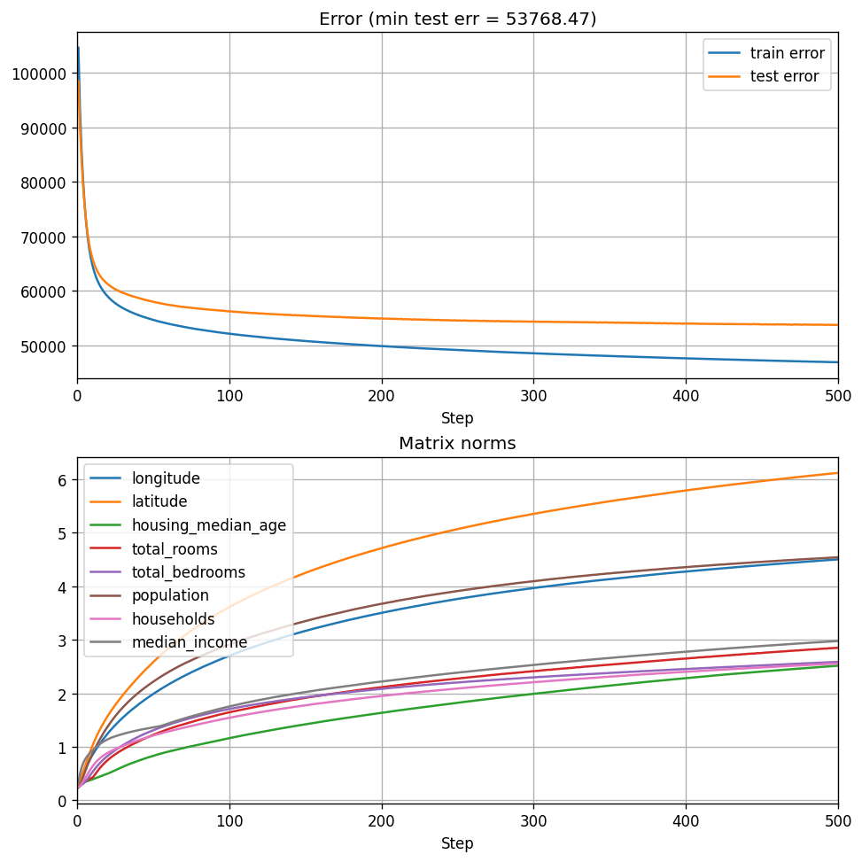
Recall that for a $30 \times 30$ matrix, we got a test error of $\approx \$54200$, so scaling up indeed improves performance somewhat, but not dramatically. Apparently, with our current training procedure we begin to notice the diminishing returns of this type of scaling.

Now, this does not mean that our training procedure is the best, and this is definitely not an exhaustive scaling experiment, where we choose the best training procedure we can, and perhaps devise some rule of hyperparameter transfer from smaller to larger models. But having the ability to compute eigenvalues quickly lets us actually conduct this research, since PyTorch eigenvalue solver was simply too slow.

Recap

Now that we have the ability to conduct fast experiments we can move forward and do other interesting stuff. Obviously, there might be even better ways to achieve our goal - perhaps writing a custom CUDA kernel for the entire function $f(\mathbf{x}; {\boldsymbol \mu}, \mathbf{A}_{1:n})$ would even be better. But I just wanted something that doesn’t get in my way when I’m experimenting - that’s all.

The next post in the series will be very different - it will be theoretical. We did a lot of practical things here, but we need to understand some things before we move forward. So stay tuned!

References

Clarke, Frank H. “Generalized gradients and applications.” Transactions of the American Mathematical Society 205 (1975): 247-262. ↩
Clarke, Frank H. Optimization and nonsmooth analysis. Society for industrial and Applied Mathematics, 1990. ↩
Park, Sejun, Sanghyuk Chun, and Wonyeol Lee. “What does automatic differentiation compute for neural networks?.” The Twelfth International Conference on Learning Representations. 2024. ↩
Bolte, Jérôme, Tam Le, and Edouard Pauwels. “Subgradient sampling for nonsmooth nonconvex minimization.” SIAM Journal on Optimization 33.4 (2023): 2542-2569. ↩ ↩²

I feel the need for Eigen-Speed

This post is part of the series "Eigenvalues as models", and is not self-contained.

Series posts:

Behold the power of the spectrum!

Robustness, interpretability, and scaling of eigenvalue models

I feel the need for Eigen-Speed (this post)

Intro

Warm-up

Eigenvalue gradients

A custom \(k\)-th eigenvalue function

Trying it out in practice

Recap

This post is part of the series "Eigenvalues as models", and is not self-contained.

Series posts:

Behold the power of the spectrum! Robustness, interpretability, and scaling of eigenvalue models I feel the need for Eigen-Speed (this post)

Intro

Warm-up

Eigenvalue gradients

A custom \(k\)-th eigenvalue function

Trying it out in practice

Recap

Behold the power of the spectrum!

Robustness, interpretability, and scaling of eigenvalue models

I feel the need for Eigen-Speed (this post)