SkLearning with Bernstein Polynomials - continued
This post is part of the series "Polynomial features in machine learning", and is not self-contained.
Series posts:
-
“Are polynomial features the root of all evil?"
-
“Keeping the polynomial monster under control"
-
“SkLearning with Bernstein Polynomials"
- SkLearning with Bernstein Polynomials - continued (this post)
-
A Bernstein SkLearn model calibrator
-
Regularization properties of polynomial bases
-
Let the polynomial monster free
-
Off with the polynomial's tail!
-
Paying attention to feature distribution alignment
- “Are polynomial features the root of all evil?"
- “Keeping the polynomial monster under control"
- “SkLearning with Bernstein Polynomials"
- SkLearning with Bernstein Polynomials - continued (this post)
- A Bernstein SkLearn model calibrator
- Regularization properties of polynomial bases
- Let the polynomial monster free
- Off with the polynomial's tail!
- Paying attention to feature distribution alignment
Intro
In the previous post we built a Scikit-Learn component that you can already integrate into your pipelines to train models whose numerical features are represented in the Bernstein basis. Feature interactions is a simple and effective feature engineering trick, and this post builds upon this knowledge and improves the component we built by introducing pairwise interactions between numerical features. This post is a direct continuation of the previous post, and I will assume that you are familiar with what we built so far. If what you see here looks like Klingon, and you don’t know Klingon, please take your time to read the posts on polynomial features from the beginning. As previously, the code is available in a notebook that you can open in Google Colab. Due to the nature of this post, the notebook extends the code from the last post with additional experiments, rather than being written from scratch.
A recap
The BernsteinTransformer component we created last time allowed us to construct a Scikit-Learn pipeline, train, and make predictions using the following simple lines of code:
categorical_features = [...] # the list of categorical feature names
numerical_features = [...] # the list of numerical feature names
my_estimator = ... # Ridge / Lasso / LogisticRegression / ...
pipeline = training_pipeline(BernsteinFeatures(), my_estimator, categorical_features, numerical_features)

pipeline.fit(train_df, train_df[label_column])
test_predictions = pipeline.predict(test_df)
We constructed pipelines of the following generic form to facilitate using polynomial bases over data in a compact interval, by first rescaling it:
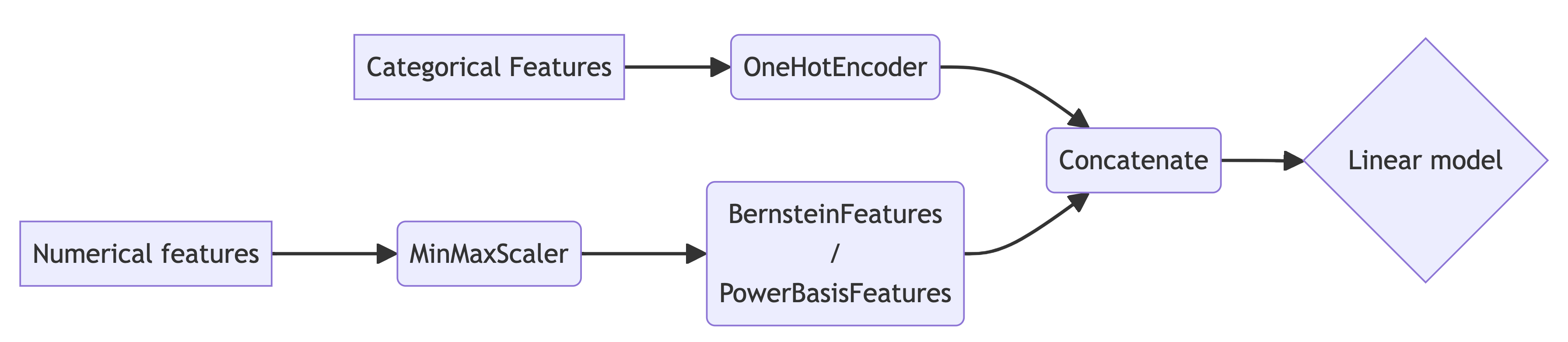
Our BernsteinTransformer generated Bernstein basis features for each column separately. As a baseline, we also used the PowerBasisTransformer that generated the power-basis features. We will extend both classes in a way that will allow us to construct pairwise interactions between numerical features by generating tensot product bases:
Such bases can be used to learn a function of any given pair of features \(x\) and \(y\) with linear coefficients:
\[f(x, y) = \sum_{i=0}^n \sum_{j=0}^n \alpha_{i,j} b_{i,n}(x) b_{j,n}(y)\]The basis \(b_{0,n}, \dots, b_{n,n}\), in this post, can be either the power-basis for n-th degree polynomials, or the Bernstein basis.
As an additional baseline, we will also Scikit-Learn’s built-int PolynomialFeatures class, that does something similar, but different with the power basis. Given \(m\) numerical features of degree \(n\), it allows learning functions of the form
\[f(x_1, \dots x_m) = \sum_{\substack{i_1 + \dots + i_m = n \\ i_k \geq 0}} \alpha_{i_1, \dots, i_m} \left( \prod_{k=1}^m x_k^{i_k} \right).\]This looks “scary”, but essentially this is a generic multivariate polynomial of degree \(n\) whose variables are \(x_1, \dots , x_m\). So let’s get started!
The pairwise interaction transformers
Without further due, let’s extend the the base-class for both polynomial feature transformers from the previous post, to have an additional interaction_features argument in its constructor, and produce tensor-product features. Again, we need to take care not to introduce an additional “bias term”, and to that end, we eliminate the first basis function, as in the previous post:
import numpy as np
from sklearn.base import BaseEstimator, TransformerMixin
from itertools import combinations


class PolynomialBasisTransformer(BaseEstimator, TransformerMixin):
    def __init__(self, degree=5, bias=False, na_value=0., interactions=False):
        self.degree = degree
        self.bias = bias
        self.na_value = na_value
        self.interactions = interactions

    def fit(self, X, y=None):
        return self

    def transform(self, X, y=None):
        # Check if X is a Pandas DataFrame and convert to NumPy array
        if hasattr(X, 'values'):
            X = X.values

        # Ensure X is a 2D array
        if X.ndim == 1:
            X = X.reshape(-1, 1)

        # Get the number of columns in the input array
        n_rows, n_features = X.shape

        # Compute the specific polynomial basis for each column
        basis_features = [
            self.feature_matrix(X[:, i])
            for i in range(n_features)
        ]

        # create interaction features - basis tensor products
        if self.interactions:
          interaction_features = [
              (u[:, None, :] * v[:, :, None]).reshape(n_rows, -1)
              for u, v in combinations(basis_features, 2)
          ]
          result_basis = interaction_features
        else:
          result_basis = basis_features

        if not self.bias:
          result_basis = [basis[:, 1:] for basis in result_basis]

        return np.hstack(result_basis)


    def feature_matrix(self, column):
      vander = self.vandermonde_matrix(column)
      return np.nan_to_num(vander, self.na_value)


    def vandermonde_matrix(self, column):
        raise NotImplementedError("Subclasses must implement this method.")
Our concrete bernstein and power basis transformers from the previous post remain the same - their job is implementing the vandermonde_matrix method. We include them here for completeness:
class BernsteinFeatures(PolynomialBasisTransformer):
    def vandermonde_matrix(self, column):
        basis_idx = np.arange(1 + self.degree)
        basis = binom.pmf(basis_idx, self.degree, column[:, None])
        return basis


class PowerBasisFeatures(PolynomialBasisTransformer):
    def vandermonde_matrix(self, column):
        return poly.polyvander(column, self.degree)
The rest of the components we built in the previous post remain the same. So let’s try them out, and add another experiment to our attempts to predict california housing prices!
California housing dataset with pairwise polynomial features
Recall, that we’re given a train and a test set already in Google colab, and can load them:
train_df = pd.read_csv('sample_data/california_housing_train.csv')
test_df = pd.read_csv('sample_data/california_housing_test.csv')
print(train_df.head())

#    longitude  latitude  housing_median_age  total_rooms  total_bedrooms  population  households  median_income  median_house_value
# 0    -114.31     34.19                15.0       5612.0          1283.0      1015.0       472.0         1.4936             66900.0
# 1    -114.47     34.40                19.0       7650.0          1901.0      1129.0       463.0         1.8200             80100.0
# 2    -114.56     33.69                17.0        720.0           174.0       333.0       117.0         1.6509             85700.0
# 3    -114.57     33.64                14.0       1501.0           337.0       515.0       226.0         3.1917             73400.0
# 4    -114.57     33.57                20.0       1454.0           326.0       624.0       262.0         1.9250             65500.0
The task is predicting the median_house_value column based on the other columns. Let’s use the same categorical and numerical features as in our previous post:
categorical_features = ['housing_median_age']
numerical_features = ['longitude', 'latitude', 'total_rooms', 'total_bedrooms', 'population', 'households', 'median_income']
target = ['median_house_value']
And use the same pipeline construction function as in the previous post:
from sklearn.linear_model import Ridge
from sklearn.compose import TransformedTargetRegressor

def california_housing_pipeline(basis_transformer):
    return training_pipeline(
        basis_transformer,
        TransformedTargetRegressor(
            regressor=Ridge(),
            transformer=MinMaxScaler()
        ),
        categorical_features,
        numerical_features
    )
So now, in addition to the linear, power basis, and Bernstein bases, we will add the pairwise power basis, pairwise Bernstein basis, and the the built-int PolynomialFeatures basis. Let’s begin with the pairwise Bernstein basis. Note the interactions=True argument I give to the BernsteinFeatures component:
inter_param_space = {
    'preprocessor__numerical__basis__degree': hp.uniformint('degree', 1, 8),
    'model__regressor__alpha': hp.loguniform('C', -10, 5)
}

bernstein_inter_pipeline = california_housing_pipeline(BernsteinFeatures(interactions=True))
tune_and_evaluate_pipeline(bernstein_inter_pipeline, inter_param_space,
                           train_df, test_df, target,
                           'neg_root_mean_squared_error')
This time we’ll use lower polynomial degrees, up to 8, because the model becomes too large to finish tuning in a few minutes on Colab. I got the following result:
Tuning params
100%|██████████| 100/100 [14:10<00:00,  8.50s/trial, best loss: 55558.90453947183]
Best params = {'model__regressor__alpha': 0.003973626254894749, 'preprocessor__numerical__basis__degree': 8}
Refitting with best params on the entire training set
Test metric = -58131.78984
Now let’s try the power basis with interactions:
power_inter_pipeline = california_housing_pipeline(PowerBasisFeatures(interactions=True))
tune_and_evaluate_pipeline(power_inter_pipeline, inter_param_space,
                           train_df, test_df, target,
                           'neg_root_mean_squared_error')
After a few minutes I get the following output:
Tuning params
100%|██████████| 100/100 [12:25<00:00,  7.46s/trial, best loss: 56765.359651797495]
Best params = {'model__regressor__alpha': 0.00017748456793637552, 'preprocessor__numerical__basis__degree': 8}
Refitting with best params on the entire training set
Test metric = -59228.75478
So we can certainly see that even with interaction features, the power basis performs worse than the Bernstein basis.
And last but not least, let’s use the PolynomialFeatures class that the Scikit-Learn package provides. To be fair, we need to choose its maximum degree so that the number of generated features is similar to that of the pairwise bases. So we have 7 numerical features, and therefore \(\frac{1}{2} \cdot 7 \cdot 6 = 21\) feature pairs. With maximum degree of 8, each pair generates at most \(8 \cdot 8 - 1 = 63\) basis functions. So the total number of generated features is \(21 \cdot 63 = 1323\).
A multivariate polynomial with \(7\) variables of degree \(d\) has
\[{7 + d \choose d}\]coefficients. It can be easily shown using the stars and bars technique in combinatorics. Choosing \(d = 7\) we get 1716 coefficients, which is pretty close. With \(d=6\) we get less than 1323 coefficients, so using polynomials of max degree 7 seems like a reasonable choice.
Let’s try it out!
from sklearn.preprocessing import PolynomialFeatures

polyfeat_param_space = {
    'preprocessor__numerical__basis__degree': hp.uniformint('degree', 1, 7),
    'model__regressor__alpha': hp.loguniform('C', -10, 5)
}


polyfeat_pipeline = california_housing_pipeline(PolynomialFeatures(include_bias=False))
tune_and_evaluate_pipeline(polyfeat_pipeline, polyfeat_param_space,
                           train_df, test_df, target,
                           'neg_root_mean_squared_error')
After a few minutes, I got the following output:
Tuning params
100%|██████████| 100/100 [25:59<00:00, 15.60s/trial, best loss: 56986.28132958403]
Best params = {'model__regressor__alpha': 0.0003080552886505334, 'preprocessor__numerical__basis__degree': 6}
Refitting with best params on the entire training set
Test metric = -59155.28068
So, summarizing the results of the previous post, together with the results of this post, we obtain the following table:
| Linear | Power basis | Bernstein basis | Pairwise Bernstein | Pairwise Power | Full polynomial | |
|---|---|---|---|---|---|---|
| RMSE | 67627.17474 | 63534.49228 | 61559.04848 | 58131.78984 | 59228.75478 | 59155.28068 |
| Improvement over Linear | 0% | 6.05% | 8.97% | 14.04% | 12.41% | 12.52% |
| Tuned degree | 1 | 31 | 50 | 8 | 8 | 6 |
As we can see, the clear winners are the pairwise polynomial features. This, of course, will not always be the case. But there is a good reason why it may be an option worth exploring.
Bernstein tensor products
Let’s get formally introduced - the set of functions \(\mathbb{B}_{n,n} = \{ b_{i,n}(x) b_{j,n}(y) \}_{i,j=0}^n\) is the tensor product basis constructed from the \(n\)-th degree Bernstein basis. In general, tensor product bases are function bases that are composed of pairwise product of basis functions, but here we explore the special case of Bernstein basis functions. The basis \(\mathbb{B}_{n,n}\) shares some nice properties with the Bernstein basis:
- Non-negativity: \(b_{i,n}(x) b_{j,n}(y) \geq 0\)
- Partition of unity: \(\displaystyle \sum_{i=0}^n \sum_{j=0}^n b_{i,n}(x) b_{j,n}(y) = 1\)
Now let’s look at an arbitrary function \(f\) that is spanned by this basis:
\[f(x,y) = \sum_{i=0}^n \sum_{j=0}^n \alpha_{i,j} b_{i,n}(x) b_{j,n}(y)\]Due to the two properties above, like in the case of the univariate Bernstein basis, \(f\) is just a weighted sum of its coefficients \(\alpha_{i,j}\). The basis function values specify the weight of each coefficient.
Moreover, we have the same ‘controlling’ property as with the univariate basis - \(\alpha_{i,j}\) “controls” the value of the function \(f\) in the vicinity of the point \((\frac{i}{n}, \frac{j}{n})\). These properties make it easy to regularize \(f\), just as in the case of the univariate basis. We will not go into the details in this post, but just as is the case with the univariate basis, we can also control the first or second derivative of \(f\) by imposing constraints on its coefficients based on discrete analogues of first and second order differences.
Despite the name ‘basis’, it is important to note that the tensor product basis does not span all bivariate polynomials of degree \(2n\), but merely a very useful subspace. For example, the monomials \(x^{2n}\) and \(y^{2n}\) appear nowhere in the polynomial expansion of the \(f(x, y)\) defined above.
Bases with such properties, such as the Bernstein basis, and also the well-known B-Spline basis are heavily used by computer aided design software to represent 2D surfaces embedded in 3D 1. In the case of the Bernstein basis, the surfaces are known as Bézier surfaces, named after the French engineer Pierre Bézier. I like the idea of propagating knowledge established in one field to another field, and I believe this is one such case. I’d like to refer interested readers to the beautiful tutorial paper2 by Michael Floater and Kai Hormann.
Summary
This post concludes our adventures in designing a Scikit-Learn transformer. I’m happy to receive feedback, so please don’t hesitate to contact me if you have feedback to share. Next, we will explore a practical case when controlling polynomial derivatives is important, and write yet another Scikit-Learn component. Stay tuned!
-
When representing a 3D surface, we have three functons \(f_x, f_y, f_z\), one for the \(x\) coordinate, one for the \(y\), and one for the \(z\) coordinate. ↩
-
Michael S. Floater & Kai Hormann Surface Parameterization: a Tutorial and Survey. Mathematics and Visualization. Springer, Berlin, Heidelberg. https://doi.org/10.1007/3-540-26808-1_9 ↩