Off with the polynomial's tail!

Intro

Last time we did a small curve fitting exercise - we fit high degree polynomials represented in the Legendre basis to a curve, and observe the celebrated “double descent” phenomenon: after crossing the memorization threshold, the generalization error improves as the degree increases. Then, we took a closer look at what happens when we fit a high degree of Legendre polynomial to try to explain this double descent. We observed that the Legendre basis polynomials oscilate, and therefore behave like a kind of a “frequency domain”, and conjectured that coefficients of lower degree functions are responsible for the overall shape of the fit curve, whereas coefficients of higher degree functions model rapid fluctuations that fit the deviation from the overall shape to the noisy data. Then, looked at “pruned” polynomials obtained by using only a few initial coefficients and discarding the rest, and indeed saw that the pruned function captures the overall shape.

In this post we shall study this phenomenon not for fitting a curve, but for fitting a regression model to our favorite dataset in this blog - the California Housing dataset. When writing this post I learned something surprising and new, and I hope to surprise you as well. This may not be a new state of the art method, but it is a surprising insight, heavily inspired by a short online discussion with Prof. Francesco Orabona about what does it mean for a model to be “simple”. In fact, this discussion is what led me to write this post.

As always, the code can be found in a notebook you can deploy to Colab and play with yourself. There will be no formulas or math in this post - mostly code and plots. So let’s get started!

Double-descent with california housing

Let’s start by preparing the data. We do some standard stuff, nothing fancy. Load the data:

import pandas as pd

train_df = pd.read_csv("sample_data/california_housing_train.csv")
test_df = pd.read_csv("sample_data/california_housing_test.csv")
train_df.head(5)

 longitude  latitude  housing_median_age  total_rooms  total_bedrooms  population  households  median_income  median_house_value
   -118.07     33.81                22.0       2711.0           352.0      1305.0       368.0         8.5407            398800.0
   -117.63     33.50                12.0       3619.0           536.0      1506.0       492.0         7.2013            353600.0
   -117.09     32.57                17.0        444.0            83.0       357.0        87.0         5.1478            138900.0
   -117.16     32.81                34.0       2275.0           375.0      1021.0       379.0         3.6371            176300.0
   -118.07     34.17                36.0       2415.0           394.0      1215.0       413.0         5.5418            326100.0

Split the loaded training set into a training and validation set:

from sklearn.model_selection import train_test_split

train_df, valid_df = train_test_split(train_df, test_size=0.2, random_state=42)

Separate the prediction target column to a separate variable:

X_train = train_df.drop("median_house_value", axis=1)
y_train = train_df["median_house_value"]

X_valid = valid_df.drop("median_house_value", axis=1)
y_valid = valid_df["median_house_value"]

X_test = test_df.drop("median_house_value", axis=1)
y_test = test_df["median_house_value"]

Finally, one can observe that there are some numerical columns ith extremely skewed distributions which are more sane after a log transformation:

import numpy as np

skewed_columns = ['total_rooms', 'total_bedrooms', 'population', 'households']
X_train.loc[:, skewed_columns] = X_train[skewed_columns].apply(np.log)
X_valid.loc[:, skewed_columns] = X_valid[skewed_columns].apply(np.log)
X_test.loc[:, skewed_columns] = X_test[skewed_columns].apply(np.log)

I want to avoid plots to convince you that these are the “skewed” columns, since this is not the objective of this post. So here you will have to trust me :)

Now let’s get to the meat. We will rely on Scikit-Learn a lot here, and in particular, on the Pipeline objects, that streamlines the data preparation before model fitting. It implements the “fit-predict” paradigm, where fitting the entire pipeline is done on the training set, and then we can do prediction. The data preparation components in a pipeline are known in Scikit-Learn as Transformer objects, since they transform data. Do not confuse them with Transformer models, used for language tasks.

So let’s write a simple transformer that converts each column in a dataset with numerical features to a corresponding Legendre Vandermonde matrix. Recall, that we relied on thenp.polynomial.legendre.legvander NumPy method in our last post, and it turns out it naturally handles datasets with multiple columns. Let’s see an example:

X = np.array([
    [0, 0.2],
    [0.4, 0.6],
    [0.8, 1]
])
print(np.polynomial.legendre.legvander(X, 4))

[[[ 1.     0.    -0.5   -0.     0.375]
  [ 1.     0.2   -0.44  -0.28   0.232]]

 [[ 1.     0.4   -0.26  -0.44  -0.113]
  [ 1.     0.6    0.04  -0.36  -0.408]]

 [[ 1.     0.8    0.46   0.08  -0.233]
  [ 1.     1.     1.     1.     1.   ]]]

The output is a 3D array - each scalar has been expanded into a vector five Legendre basis values, corresponding to the five basis functions of degree 4.

But to fit a model we don’t need a 3D array, but a 2D array - the rows are the samples, and the columns are the features. So all we need to do is squeeze the last two dimensions using a simple reshape operation - it will automatically horizontally concatenate the Legendre features from each column:

print(np.polynomial.legendre.legvander(X, 4).reshape(4, -1))

[[ 1.     0.    -0.5   -0.     0.375  1.     0.2   -0.44  -0.28   0.232]
 [ 1.     0.4   -0.26  -0.44  -0.113  1.     0.6    0.04  -0.36  -0.408]
 [ 1.     0.8    0.46   0.08  -0.233  1.     1.     1.     1.     1.   ]]

Now we see two “blocks” of Legendre Vandermonde matrices, concatenated horizontally - one block for every column. Each block has 5 columns, corresponding to the five basis functions of degree 4.

Finally, note that we have a column of ones - this column is the “bias” term of each polynomial. But we don’t want a bias term for every polynomial - we want one bias term for the entire model. So we will have to remove these columns of ones, and let the linear regression model in Scikit-Learn have its own bias. Now we’re ready to write our transformer. There is some boilerplate, but everything substantial I already explained above.

from sklearn.base import TransformerMixin, BaseEstimator

class LegendreScalarPolynomialFeatures(TransformerMixin, BaseEstimator):
    def __init__(self, degree=2, include_bias=False):
        self.degree = degree
        self.include_bias = include_bias

    def fit(self, X, y=None):
        # There is nothing to learn
		# Legendre polynomials do not depend on the training data.
        return self

    def __sklearn_is_fitted__(self):
        # See above - it's always "fitted" by definition
        return True

    def transform(self, X, y=None):
        # Make sure X is of the right type and shape
        X = check_array(X, accept_sparse=False, ensure_all_finite=True)

        # create a Vandermonde matrix for each feature, and create a 3D array
        # of shape
        vander = np.polynomial.legendre.legvander(X, self.degree)
        if not self.include_bias:
            # discard the column of ones for each feature
            vander = vander[..., 1:] 

        # reshape to concatenate the Vandermonde matrices horizontally
		n_rows = X.shape[0]
        result = vander.reshape(n_rows, -1)
        return result

Let’s try it out:

LegendreScalarPolynomialFeatures(degree=4).transform(X)

[[ 0.    -0.5   -0.     0.375  0.2   -0.44  -0.28   0.232]
 [ 0.4   -0.26  -0.44  -0.113  0.6    0.04  -0.36  -0.408]
 [ 0.8    0.46   0.08  -0.233  1.     1.     1.     1.   ]]

The same matrix we saw before, but without the columns of ones.

Let’s see how we can use our new shiny component inside a Scikit-Learn pipeline. Our pipeline will first scale the features to be in the range \([-1, 1]\), so that we are in the in the “operating region” of the Legendre basis, then it will convert the scaled features to Legendre polynomials using our component, and finally it will fit a simple linear regression model. Here is how we can build such a pipeline for polynomials of degree 8:

from sklearn.preprocessing import MinMaxScaler
from sklearn.linear_model import LinearRegression
from sklearn.pipeline import Pipeline

pipeline = Pipeline([
        ('minmaxscaler', MinMaxScaler(feature_range=(-1, 1), clip=True)),
        ('polyfeats', LegendreScalarPolynomialFeatures(degree=8)),
        ('model', LinearRegression()),
    ])

The pipeline is simply composed of a sequence of steps, associated with a name of our choice. Here is how we fit it on the training data, and then compute the test error:

pipeline.fit(X_train, y_train)
test_error = root_mean_squared_error(y_test, pipeline.predict(X_test))
print(f'Test error = {test_error:.4f}')

Test error = 63475.8142

It appears large, but we’re dealing here with sums of money representing housing prices - hundreds of thousands of dollars. So it’s not that large.

Now let’s try to reproduce our double descent. We will iterate over several degrees, fit a pipeline to the training data, and compute the test errors. Note, that we compute test errors and not validation errors, because we care about observing the generalization power, and not tuning some parameter. Moreover, to make it run in a reasonable time, we sample a subset of the training set - 5000 out of the 13700 rows. Here is the code:

degrees = list(range(1, 10)) + np.geomspace(10, 40000, 12).astype(np.int32).tolist()
train_rmses = []
test_rmses = []

# sample training set - note that it's already randomly permuted
# by the train-test split.
n_samples = 5000
X_train_samples = X_train.iloc[:n_samples, :]
y_train_samples = y_train.iloc[:n_samples]

# fit various degrees
for degree in degrees:
    pipeline = Pipeline([
        ('minmaxscaler', MinMaxScaler(feature_range=(-1, 1), clip=True)),
        ('polyfeats', LegendreScalarPolynomialFeatures(degree=degree)),
        ('model', LinearRegression())
    ])
    pipeline.fit(X_train_samples, y_train_samples)
    y_train_pred  = pipeline.predict(X_train_samples)
    y_test_pred = pipeline.predict(X_test)

    train_rmses.append(root_mean_squared_error(y_train_samples, y_train_pred))
    test_rmses.append(root_mean_squared_error(y_test, y_test_pred))
    print(f"Degree: {degree}, "
          f"Test RMSE: {test_rmses[-1]:.2f}, "
          f"Train RMSE {train_rmses[-1]:.2f}")

Degree: 1, Test RMSE: 68326.20, Train RMSE 66776.99
Degree: 2, Test RMSE: 67522.42, Train RMSE 65720.98
Degree: 3, Test RMSE: 65784.84, Train RMSE 64030.37
Degree: 4, Test RMSE: 65227.71, Train RMSE 63353.57
Degree: 5, Test RMSE: 64907.57, Train RMSE 62297.19
Degree: 6, Test RMSE: 65134.09, Train RMSE 62006.36
Degree: 7, Test RMSE: 64675.77, Train RMSE 61721.51
Degree: 8, Test RMSE: 64534.99, Train RMSE 61459.37
Degree: 9, Test RMSE: 64962.61, Train RMSE 61285.31
Degree: 10, Test RMSE: 64433.99, Train RMSE 60810.69
Degree: 21, Test RMSE: 1701699.31, Train RMSE 57939.34
Degree: 45, Test RMSE: 2786592773542.82, Train RMSE 55145.90
Degree: 96, Test RMSE: 24926913710269.14, Train RMSE 50786.59
Degree: 204, Test RMSE: 6879185912413.60, Train RMSE 47511.24
Degree: 433, Test RMSE: 5893934722602.69, Train RMSE 41896.23
Degree: 922, Test RMSE: 1642004977035.12, Train RMSE 32491.25
Degree: 1959, Test RMSE: 295197737240.98, Train RMSE 14681.05
Degree: 4165, Test RMSE: 116144.54, Train RMSE 0.00
Degree: 8854, Test RMSE: 85373.33, Train RMSE 0.00
Degree: 18819, Test RMSE: 78639.33, Train RMSE 0.00
Degree: 40000, Test RMSE: 75965.36, Train RMSE 0.00

We see a nice double descent! The train error goes down towards zero. The test error first increases with the degree, and then decreases again! It is not obvious where the “memorization threshold” is now, since the features are correlated. For example, total rooms and total bedrooms are correlated:

np.corr(X_train["total_rooms"], X_train["total_bedrooms"])

[[1.         0.94465316]
 [0.94465316 1.        ]]

This means, for instance, that the block of Legendre features for total bedrooms does not necessarily add more information. Thus, it’s not very trivial where this “memorization threshold” is in terms of the polynomial degree. But it is somewhere between 1959 and 4165, since we see that the train error drops to zero somewhere in between.

We can also plot the double descent curve using the train and test errors we just stored:

fig, ax = plt.subplots()
ax.plot(degrees, train_rmses, label="Train")
ax.plot(degrees, test_rmses, label="Test")
ax.set_ylim([-0.1, 2 * np.max(test_rmses)])
ax.set_ylabel("RMSE")
ax.set_xscale('log')
ax.set_xlabel("Polynomial degree")
ax.set_yscale('asinh')
ax.legend()

fig.show()

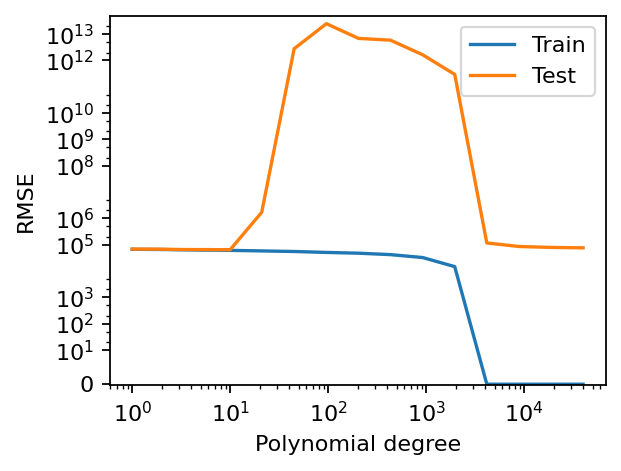
It’s interesting to see that the test error of polynomial features of degree 40,000 is quite small, but it it’s worse than that if the low degree polynomials. I’m pretty sure that if we crank up the degree to a few millions it will be better, but that would be an overkill. Having demonstrated the double descent, I want to take this post in a different direction.

Pruning

First, let’s see if pruning the “tail” of the polynomial even makes sense - meaning that higher degrees simply add more intricate details to an already well-formed polynomial. To that end, let’s plot the polynomial we obtained for each feature by taking only the first \(k\) coefficients, for various values of \(k\).

Recall, that our pipeline has a step named model, which is a linear regression model. We can access its coefficients:

lin_reg = pipeline.named_steps['model']
print(lin_reg.coef_.shape)

(320000,)

We see that we have exactly \(8 \times 40{,}000 = 320{,}000\) coefficients. This is because we have 8 columns, each represented by 40,000 coefficients of a polynomial of degree 40,000 without its bias term. We can access the coefficients of each polynomial by reshaping these coefficients into a matrix of 8 rows. This is exactly what the following function does - extracts the coefficient matrix, with a row of coefficients for each feature:

def get_feature_coefs(pipeline):
    num_features = pipeline.named_steps['minmaxscaler'].n_features_in_
    lin_reg = pipeline.named_steps['model']
    feature_coefs = lin_reg.coef_.reshape(num_features, -1)
    return feature_coefs

Now we can use it to plot the coefficients of each feature. We call the coefficients vector a spectrum, because Legendre polynomials model oscilations, just like sines and cosines.

def plot_spectra(pipeline):
    feature_coefs = get_feature_coefs(pipeline)

    # define subplots for each feature
    n_cols = 3
    n_rows = math.ceil(feature_coefs.shape[0] / n_cols)
    width, height = plt.rcParams['figure.figsize']
    fig, axs = plt.subplots(
        n_rows, n_cols, figsize=[n_cols * width, n_rows * height],
        sharex=True,
        layout='constrained')

    # plot coefficients
    for i, (coef_vec, ax) in enumerate(zip(feature_coefs, axs.ravel())):
        ax.plot(coef_vec)
        ax.set_title(f'{X_train.columns[i]}')

    fig.show()

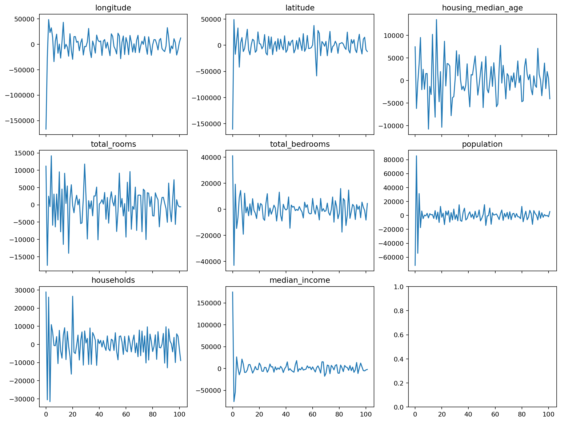
plot_spectra(pipeline)

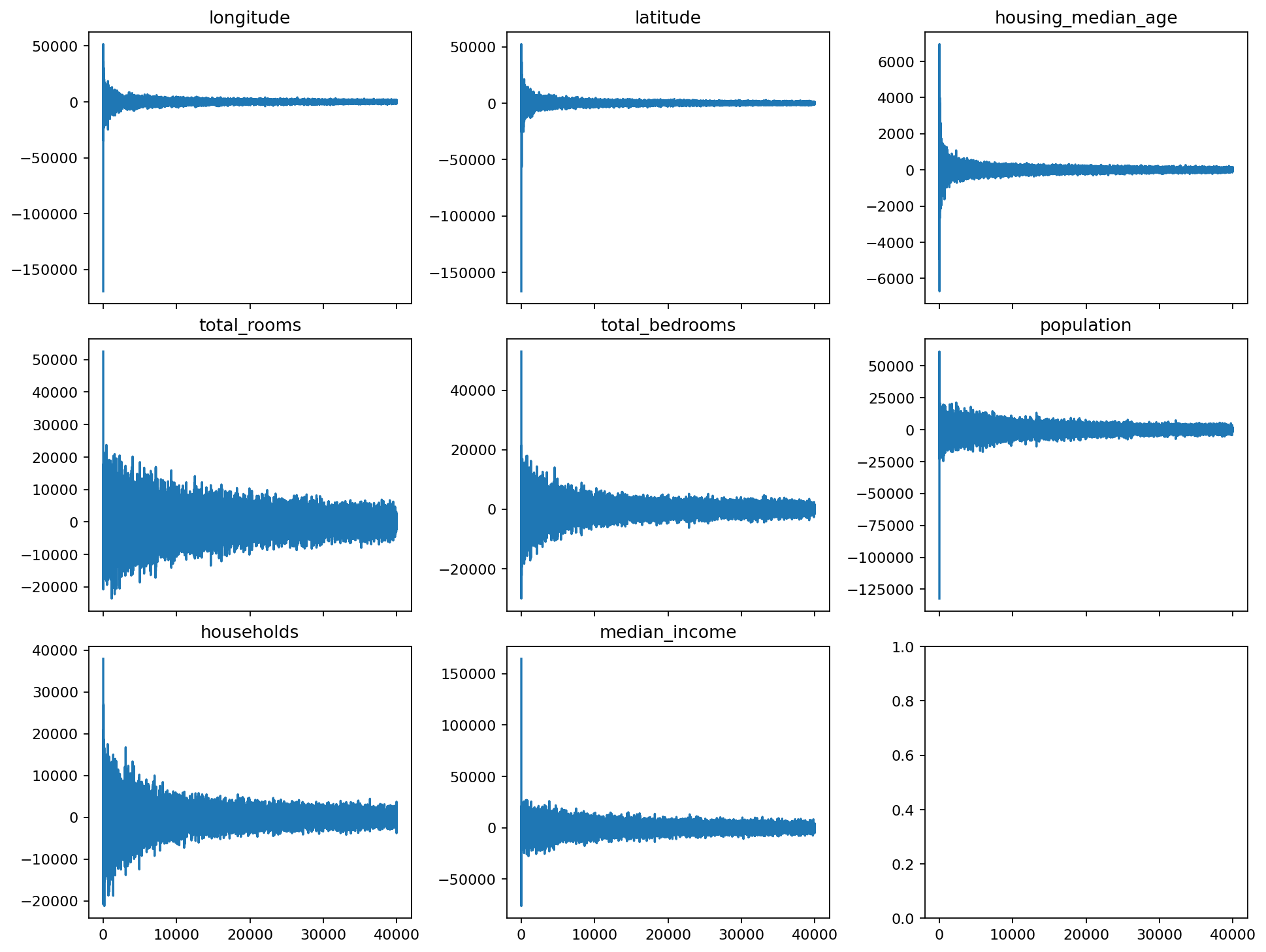
Indeed, for each one of the features the coefficients “decay” towards zero. There are features where it happens quickly, and those where it happens slowly, but it happens for all of them. So “pruning” makes sense - we remove fine details modeled by the rapid oscillations of the high degree polynomials, and remain with the overall shape.

So let’s define a function that prunes each polynomial by preserving only the initial \(k\) coefficients for several values of \(k\), and see the results. The function is a bit lengthy due to boilerplate, but pretty straightforward:

def plot_feature_curves(
        pipeline, pruned_degrees=[1, 2, 3, 5, 10, 20, 2000], plot_resolution=5000
):
    # extract coefficients of each feature from the model
    feature_coefs = get_feature_coefs(pipeline)
    num_features = feature_coefs.shape[0]

    # define grid of plots for features x degrees
    width, height = plt.rcParams['figure.figsize']
    fig, axs = plt.subplots(
        feature_coefs.shape[0], len(pruned_degrees),
        layout='constrained', sharex=True, sharey='row',
        figsize=(width * len(pruned_degrees) / 3, height * num_features / 3))

    # compute Legendre Vandermonde matrix of maximum degree, to be pruned
    x_plot = np.linspace(0, 1, plot_resolution)
    full_vander = np.polynomial.legendre.legvander(x_plot, max(pruned_degrees))

    # do the plotting for each feature and degree
    for feat in range(num_features):
        for i, degree in enumerate(pruned_degrees):
            # prune coefficients of current feature at current degree
            pruned_coefs = feature_coefs[feat, :1 + degree]

            # prune Vandermonde matrix up to current degree
            pruned_vander = full_vander[:, :1 + degree]

            # plot the current degree polynomial
            y_plot = pruned_vander @ pruned_coefs
            axs[feat, i].plot(x_plot, y_plot)

            # put axis titles
            if feat == 0:
                axs[feat, i].set_title(f"deg={degree}")
            if i == 0:
                feature_name = X_train.columns[feat].replace("_", "\n")
                axs[feat, i].set_ylabel(feature_name)

    fig.align_ylabels(axs[:, 0])
    fig.show()

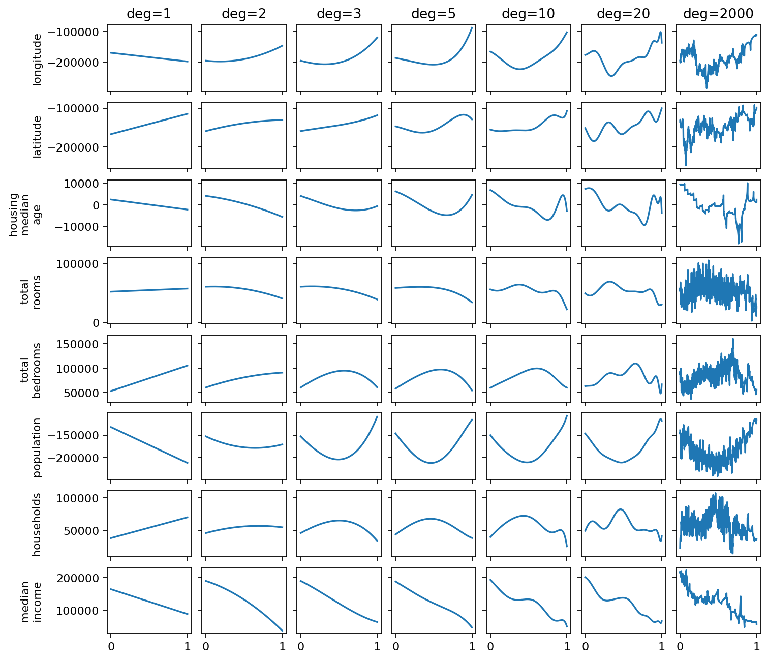
We can see some interesting things. For example, for the population feature, the polynomial of degree 3 captures the overall shape quite well. For the median income, the lower degrees also do quite a good job. Moreover, we see that we have more oscillations that look like noise added on top of the overall shape for some of the features, notably, total rooms, total bedrooms, population, and households. These are exactly the features for which the spectrum decays slowly - higher degrees that model rapid oscillations have a larger effect.

So here comes an interesting conjecture - maybe keeping just the “overall shape” by pruning the higher order coefficients we can achieve an even better generalization error? Well, let’s put it to a test! Here is a small function that takes a pipeline, and creates a new one of a lower degree with pruned coefficients. The code is quite straightforward - just remove the “tail” of coefficients, and make the polynomials of the corresponding degree:

def prune_pipeline(pipeline, pruned_deg):
    pruned = deepcopy(pipeline)
    num_features = pruned.named_steps['minmaxscaler'].min_.shape[0]
    orig_degree = pruned.named_steps['polyfeats'].degree
    pruned.named_steps['polyfeats'].degree = pruned_deg

    lin_reg = pruned.named_steps['model']
    orig_coef = lin_reg.coef_.reshape(num_features, orig_degree)
    pruned_coef = orig_coef[:, :pruned_deg].ravel()
    lin_reg.coef_ = pruned_coef
    lin_reg.n_features_in_ = pruned_coef.shape[0]

    return pruned

Now we can create degree-pruned pipelines, select the degree giving us the smallest validation error, and compute the test error. Note, that this is the first time we’re using our validation set, because here we are actually tuning a parameter - we are tuning the pruned pipeline’s degree:

# get a set of degrees to try pruning at.
prune_degrees = np.concatenate([
    np.arange(1, 100),
    np.geomspace(100, 5000, 50).astype(np.int32)
])

# compute validation error for each pruned degree
pruned_errors = np.zeros(len(prune_degrees))
for i, degree in enumerate(prune_degrees):
    pruned = prune_pipeline(pipeline, degree)
    y_valid_pred = pruned.predict(X_valid)
    pruned_errors[i] = root_mean_squared_error(y_valid, y_valid_pred)
    
# compute the test error for the optimal degree
best_degree = prune_degrees[np.argmin(pruned_errors)]
pruned = prune_pipeline(pipeline, best_degree)
pruned_test_error = root_mean_squared_error(y_test, pruned.predict(X_test))
print(f'Best degree = {best_degree}, test error = {pruned_test_error}')

Best degree = 100, test error = 60014.842969972255

Much better than the test error we obtained with pure fitting! When we plotted the double descent curve, the best test error was obtained for a polynomial of degree 8, and it was 64534.99. That’s a very nice improvement of approximately 7% in RMSE!

Obviously, we could also try a regularized fit, and tune the regularization coefficient. It may even yield a better generalization error, but this misses the point. Here, it is a post fitting procedure. We first fit a model, without tuning anything, and then tune it by pruning coefficients. A lot of coefficients! We reduce the model from being a polynomial of degree 40,000 to a polynomial of degree 100!

Let’s plot the validation error as a function of the pruned degree, and also add the original best test error, the best pruned validation error, and the best pruned test error to the plot:

plt.plot(prune_degrees, pruned_errors, label='Pruned valid')
plt.xlabel("Pruned degree")
plt.ylabel("Test RMSE")
plt.xscale('asinh')
plt.axhline(np.min(pruned_errors), linestyle='--',
            label=f'Best pruned: {np.min(pruned_errors):.3f}', color='orange')
plt.axhline(pruned_test_error, linestyle='--',
            label=f'Best pruned test: {pruned_test_error:.3f}', color='red')
plt.axhline(np.min(test_rmses), linestyle='--',
            label=f'Best fit: {np.min(test_rmses):.3f}', color='navy')
plt.legend()
plt.show()

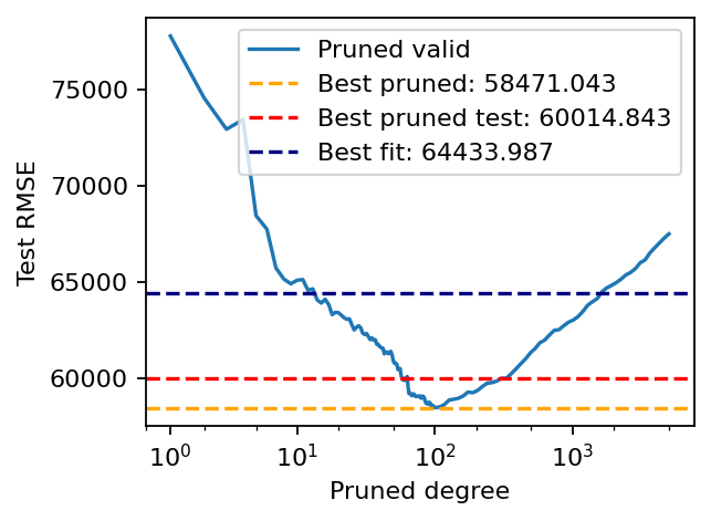
The blue curve shows us that pruning the polynomials to a degree of approximately 100 is a good choice in terms of the validation error. The corresponding test error is shown in red. For comparison, the test error obtained by fitting a polynomial of degree 8 is in blue.

Intuitively, it appears that fitting polynomials of higher degrees lets the model separate “signal” from “noise”, and by pruning we remove the noise and stay with the signal. It’s not a rigorous analysis, but it’s an intuition that appears to make sense given the decaying spectrum and the fact that we saw visually that lower degree polynomials indeed capture the high level shape. The fact that Legendre polynomials act like a frequency spectrum lets us “distil” the simple model hiding inside the highly overparameterized model explicitly. It’s not even hiding - it’s in plain sight, in the lower-degree coefficients.

So let’s take it one step further. We can actually do some greedy pruning of the polynomial of each feature separately using our validation set. Since it’s convenient that all polynomials are of the same degree, so we can store them in a matrix, we will do the pruning by zeroing out the corresponding tail of coefficients for each feature. Here is a function that prunes the degree of one given feature by zeroing the tail coefficients. The code is quite straightforward:

def prune_feature(pipeline, feature, pruned_deg):
    pruned = deepcopy(pipeline)
    num_features = pruned.named_steps['minmaxscaler'].n_features_in_
    full_deg = pruned.named_steps['polyfeats'].degree

    regressor = pruned.named_steps['model']
    coef = regressor.coef_.reshape(num_features, full_deg)
    coef[feature, (1 + pruned_deg):] = 0
    regressor.coef_ = coef.ravel()

    return pruned

Now we can loop over a set of polynomial degrees for each feature, and select the degree that gives the best validation error:

pruned_pipeline = prune_pipeline(pipeline, 200)
degrees_to_try = range(0, 200)

for feature in range(X_train.shape[1]):
    best_deg = 0
    best_error = np.inf
    for deg in degrees_to_try:
        candidate = prune_feature(pruned_pipeline, feature, deg)
        pred = candidate.predict(X_valid)
        error = root_mean_squared_error(y_valid, pred)
        if error <= best_error:
            best_error = error
            best_deg = deg

    print(f"Best degree for feature {X_train.columns[feature]}: {best_deg}, validation error: {best_error}")
    pruned_pipeline = prune_feature(pruned_pipeline, feature, best_deg)

Best degree for feature longitude: 188, validation error: 59310.36603502216
Best degree for feature latitude: 198, validation error: 59302.68099683055
Best degree for feature housing_median_age: 16, validation error: 59072.43414192942
Best degree for feature total_rooms: 23, validation error: 58793.32412447594
Best degree for feature total_bedrooms: 34, validation error: 58246.908681064
Best degree for feature population: 6, validation error: 57845.32710297523
Best degree for feature households: 14, validation error: 57614.71621402189
Best degree for feature median_income: 8, validation error: 56791.08354124084

We can see that some features need higher degrees to represent the right overall shape, whereas others work well with lower degrees. This simple post-training procedure lets us actually customize the polynomial degree of each feature separately! Now let’s see the test error:

test_error = root_mean_squared_error(y_test, candidate.predict(X_test))
print("Best pipeline test error: ", test_error)

Best pipeline test error:  59497.31961895119

It appears we squeezed an additional half a percent. The test error went down from 60014.84 to 59497.32 by customizing the right degree for each feature.

Comparing to regularized regression

Pruning is all nice, but don’t we all learn to actually use regularization and tune the regularization coefficient? Well, let’s try this as well. It’s quite simple - construct a similar pipeline with a Ridge regression object, that adds L2 regularization to least-squares regression. Then, tune both the regularization coefficient and the degree of the polynomials using HyperOpt, which is a pretty good hyperparameter tuner that comes preinstalled with Colab. First, we define a function that creates a pipeline with Ridge regression model given a polynomial degree and the regularization coefficient:

from sklearn.linear_model import Ridge

def make_ridge_pipeline(degree, alpha):
    pipeline = Pipeline([
        ('minmaxscaler', MinMaxScaler(feature_range=(-1, 1), clip=True)),
        ('polyfeats', LegendreScalarPolynomialFeatures(degree=degree)),
        ('model', Ridge(alpha=alpha)),
    ])
    return pipeline

Now, to employ HyperOpt, we define a function that computes the quality of a set of hyper parameters by fitting a model and evaluating it on a validation set. While defining it, we annotate each hyperparameter with how it should be searched - degrees are search uniformly, whereas regularization coefficients are searched in log-space. Finally invoke HyperOpt’s fmin function that is going to search the space for the best hyperparameters. Here is the code:

from hyperopt import hp, fmin, tpe

def score(
        degree: hp.uniformint('degree', 1, 500),
        alpha: hp.loguniform('alpha', np.log(1e-3), np.log(1e3))
):
    pipeline = make_ridge_pipeline(degree, alpha)
    pipeline.fit(X_train_samples, y_train_samples)
    y_pred = pipeline.predict(X_valid)
    error = root_mean_squared_error(y_valid, y_pred)
    return error

best_params = fmin(
    score, space='annotated', algo=tpe.suggest, max_evals=500,
    rstate=np.random.default_rng(42)
)

print(best_params)

The fmin function shows a progress bar of the 500 trials, which took approximately four minutes, and then we print the best parameters:

100%|██████████| 500/500 [04:04<00:00,  2.05trial/s, best loss: 57888.41179388089]
{'alpha': np.float64(8.319252707439558), 'degree': np.float64(102.0)}

We see that our hyperparameter search polynomials of degree 102 - so the Ridge regression isn’t afraid of high degree polynomials either 😀. What about the test error? Let’s fit a model with the best hyperparameters, and compute the test error:

best_degree = int(best_params['degree'])
best_alpha = best_params['alpha']
best_pipeline = make_ridge_pipeline(best_degree, best_alpha).fit(X_train_samples, y_train_samples)

test_error = root_mean_squared_error(y_test, best_pipeline.predict(X_test))
print(f'Test error = {test_error:.4f}')

Test error = 59598.0548

Very close to what we achieved with pruning. So our pruned model is not bad at all, and can be seen as a reasonable baseline.But wait - we have a pretty high degree polynomial here as well. It’s not of degree 40,000, but “only” 102, but it’s still high. Maybe we can further improve the model by applying the same pruning trick to the regularized model?

Just for the sake of it - let’s look how the spectra of the polynomials the regularized model learned look like.

plot_spectra(best_pipeline)

At first glance the bahavior seems similar - the coefficients decay towards zero, some more rapidly, some slower. Now let’s prune the model to see what happens to our test error, by applying the same per-feature pruning logic we had before:

degrees_to_try = range(0, best_degree)
pruned_pipeline = deepcopy(best_pipeline)

for feature in range(X_train.shape[1]):
    best_deg = 0
    best_error = np.inf
    for deg in degrees_to_try:
        candidate = prune_feature(pruned_pipeline, feature, deg)
        pred = candidate.predict(X_valid)
        error = root_mean_squared_error(y_valid, pred)
        if error <= best_error:
            best_error = error
            best_deg = deg

    print(f"Best degree for feature {X_train.columns[feature]}: {best_deg}, validation error: {best_error}")
    pruned_pipeline = prune_feature(pruned_pipeline, feature, best_deg)

Best degree for feature longitude: 100, validation error: 57886.75083218771
Best degree for feature latitude: 99, validation error: 57884.23600560439
Best degree for feature housing_median_age: 77, validation error: 57832.46845479303
Best degree for feature total_rooms: 1, validation error: 57258.77663424223
Best degree for feature total_bedrooms: 13, validation error: 56978.72710952217
Best degree for feature population: 27, validation error: 56673.91509748052
Best degree for feature households: 27, validation error: 56453.035725897564
Best degree for feature median_income: 8, validation error: 56142.80647476099

Note something interesting - the total rooms feature got a linear function, it’s degree is one. But the total bedrooms feature got a polynomial of degree 13. We saw before that these two features are highly correlated - so remembering a lot of parameters for both of them, intuitively, wouldn’t make sense. It’s just a conjecture, since I don’t have a formal proof, but I believe that the correlation between these two features we saw before is what made the regularized Ridge model “choose” to put the overall slope into the total rooms polynomial, and the finer details into the total bedrooms polynomial.

What about the test error?

test_error = root_mean_squared_error(y_test, pruned_pipeline.predict(X_test))
print(f'Test error = {test_error:.4f}')

Test error = 58598.2801

Nice! We just reduced it from 59598.05 to 58598.28, by 1000 dollars, just by using the fact that the Legendre basis acts like a frequency spectrum whose higher frequencies can be pruned.

Summary

The idea of truncating the spectrum of a function is, of course, not new. It probably dates back to Fourier, and his celebrated Fourier series. Of course, Fourier series are a great fit for periodic functions, such as models as a function of the time of day. But it may not be a very good fit for a generic feature that exhibits no periodic nature.

Legendre polynomials are one example of a non-periodic “spectrum” composed of orthogonal functions. We pointed out in the previous post that Chebyshev polynomials are another famous example. The ideas of using these bases to represent solutions of differential equations are abundant in science and engineering, and this post partially drew inspiration from the phenomenal course of Prof. Nick Trefethen “Approximation Theory and Approximation Practice”, and his famous book¹ by the same name. Another great reference is John P. Boyd’s book ² on spectral methods for differential equations. If you weren’t yet exposed to these subjects - I assure you a fun and enlightening experience. There is plenty of things the numerical analysis community studied thoroughly that you might find interesting.

The ideas of representing by truncating a series of orthogonal functions is abundant in signal processing, and entire research streams on signal and image denoising were built on top of this idea. What we did here was just drawing some inspiration from other scientific fields into machine learning. In some sense, we “denoised” the high degree polynomials by truncating them to lower degrees. And we saw it in two different contexts - without explicit regularization, relying on double-descent with extremely high degrees, and with explicit regularization, when the degrees are lower. In both cases - the idea is the same.

The idea here is by no means the best way to build a simple model with polynomial features, and it may be the case that a more thorough attempt to fit a regularized model may yield a better test error. However, the objective of this post is different - it’s gaining a new insight. It’s understanding that over-parametrization is what lets the model learn, automatically, to separate signal from noise. That the Legendre polynomial basis lets us elicit this separation explicitly - by observing that the fit model has a decaying coefficient spectrum that can be “denoised”. This wonderful property let us extract the simple model hiding inside the over-parametried model. And it is exactly this insight that will take us to the next posts in this series!

---

References

1. Trefethen, L. N. (2019). Approximation theory and approximation practice, extended edition. Society for Industrial and Applied Mathematics. ↩

2. Boyd, J. P. (2001). Chebyshev and Fourier spectral methods. Courier Corporation. ↩