Cheaper eigenvalue training and inference

Intro

In the last post we discussed the meaning of our model family

\[f({\boldsymbol x};{\boldsymbol A}_{0..n}) = \lambda_k \Bigl({\boldsymbol A}_0 + \sum_{i=1}^n x_i {\boldsymbol A}_i\Bigr),\]

where each \(\boldsymbol A_i\) is a symmetric matrix. In the last post we discussed what these models predict, and how we can explain them to ourselves and other stakeholders. Before that, we also discussed GPU acceleration to make training and inference faster. Speed is important, but so is cost, and fast GPUs may be expensive. Here, our aim is not only to make it faster, but also cheaper, by making the eigenvalue problem easier to solve even on weaker hardware. We certainly should not be paying for a GPU and waiting more than 5 minutes to train one neuron on a tabular dataset with about 20k rows, even if this one neuron is a fairly complex one! We begin our exploration from theory, which immediately yields practical applications. And as always, we have a notebook to reproduce all experiments in this post.

Simultaneous simplification

Recall that for any orthogonal matrix \({\boldsymbol Q} \in \mathbb{R}^{d \times d}\), we have

\[\lambda_k(\boldsymbol A) = \lambda_k({\boldsymbol Q}^T \boldsymbol A {\boldsymbol Q}),\]

So our model family is invariant under such orthogonal similarity transformations, meaning a model with matrices \(\boldsymbol A_i\) is identical to a model with matrices \(\boldsymbol Q^T \boldsymbol A_i \boldsymbol Q\) for any orthogonal \(\boldsymbol Q\).

One of the interesting phenomena in linear algebra is simultaneous diagonalization. A set of matrices \({\boldsymbol A}_i\) is simultaneously diagonalizable if there exists an orthogonal matrix \({\boldsymbol Q}\) such that \({\boldsymbol Q}^T {\boldsymbol A}_i {\boldsymbol Q}\) is diagonal for all \(i\). In other words, the same matrix \(\boldsymbol Q\) diagonalizes all matrices simultaneously.

If we restrict ourselves to models where all of our learned matrices are simultaneously diagonalizable, we can just assume all matrices are diagonal:

\[f({\boldsymbol x};{\boldsymbol A}_{0:n}) = \lambda_k \Bigl(\operatorname{diag}({\boldsymbol a}_0) + \sum_{i=1}^n x_i \operatorname{diag}({\boldsymbol a}_i)\Bigr).\]

So what is the \(k\)-th eigenvalue of this matrix? It’s just the \(k\)-th smallest entry of the vector

\[{\boldsymbol a}_0 + \sum_{i=1}^n x_i {\boldsymbol a}_i.\]

On the one hand, it’s an extremely easy eigenvalue problem. But we actually lost almost all of the expressive power, since it’s just a convoluted way to describe a piecewise linear function of \({\boldsymbol x}\). We have ReLU networks for that.

But there is another family of matrices for which the eigenvalue problem is easy - symmetric tridiagonal matrices, meaning, matrices of the form:

\[\mathcal{T}(\boldsymbol a, \boldsymbol b) = \begin{pmatrix} a_1 & b_1 & 0 & \dots & 0 \\ b_1 & a_2 & b_2 & \dots & 0 \\ 0 & b_2 & a_3 & \ddots & \vdots \\ \vdots & \vdots & \ddots & \ddots & b_{n-1} \\ 0 & 0 & \dots & b_{n-1} & a_n \end{pmatrix}.\]

Such a matrix is defined by two vectors, the main diagonal \(\boldsymbol a \in \mathbb{R}^d\), and the off-diagonal \(\boldsymbol b \in \mathbb{R}^{d-1}\). Turns out this family strikes a nice balance - eigenvalues of such matrices are efficient to compute, while remaining fairly expressive. Efficiency comes from standing on the shoulders of giants, and using decades of numerical analysis research, given to us in the form of scipy.linalg.eigh_tridiagonal on a silver platter.

To appreciate the speed difference, let’s time eigenvalue and eigenvector computation using SciPy for regular dense matrices, and compare it to tridiagonal matrices. Let’s create a batch of dense matrices:

import scipy.linalg as sla
import numpy as np

# batch of 50 matrices of size 100x100
M = np.random.randn(50, 100, 100)

If you recall from previous posts - we need eigenvectors, in addition to eigenvalues, to compute gradients to train. Now let’s measure eigenvalue and eigenvector computation time. Here it is for eigenvalues:

%%timeit -n 100 -r 30
sla.eigvalsh(M, subset_by_index=(50, 50)).sum()  # 50-th eigenvalue

32.7 ms ± 4.42 ms per loop (mean ± std. dev. of 30 runs, 100 loops each)

Here it is for eigenvectors:

%%timeit -n 100 -r 30
vals, vecs = sla.eigh(M, subset_by_index=(50, 50))
vecs.sum()

34.5 ms ± 4.5 ms per loop (mean ± std. dev. of 30 runs, 100 loops each)

Alright. Now let’s do it for tridiagonal matrices. First, we generate diagonal and off-diagonal vectors:

# A batch of 50 diagonal and 50 off-diagonal vectors for 100x100 matrices.
d = np.random.randn(50, 100)
e = np.random.randn(50, 99)

Now let’s measure. Here is eigenvalue measurement:

%%timeit -n 100 -r 30
sla.eigvalsh_tridiagonal(d, e, select='i', select_range=(50, 50)).sum()

5.11 ms ± 60.1 µs per loop (mean ± std. dev. of 30 runs, 100 loops each)

Here is eigenvector measurement:

%%timeit -n 100 -r 30
vals, vecs = sla.eigh_tridiagonal(d, e, select='i', select_range=(50, 50))
vecs.sum()

6.68 ms ± 105 µs per loop (mean ± std. dev. of 30 runs, 100 loops each)

Between 5x and 6x speedup! Speed is not all we need - we also need representation power, which we shall explore in the next section.

Tridiagonal eigenvalue functions

In the last post, we saw that we can re-write our eigenvalue models as optimization problems over quadratic functions:

\[f({\boldsymbol x};{\boldsymbol A}_{0:n}) = \max_{ {\boldsymbol C} \in \mathbb{R}^{(k-1)\times d}} \min_{ {\boldsymbol u} \in \mathbb{R}^d} \left\{ {\boldsymbol u}^T \mathcal{A}(\boldsymbol x) {\boldsymbol u} : \| {\boldsymbol u} \|_2 = 1, \, {\boldsymbol C}{\boldsymbol u} = {\boldsymbol 0}\right\},\]

where

\[\mathcal{A}(\boldsymbol x) = {\boldsymbol A}_0 + \sum_{i=1}^n x_i {\boldsymbol A}_i.\]

So we have a latent variable \(\boldsymbol u\) that appears in the quadratic function \({\boldsymbol u}^T \mathcal{A}(\boldsymbol x) \boldsymbol u\), which expresses interactions between all entry pairs \(\boldsymbol u\), since:

\[{\boldsymbol u}^T \mathcal{A}(\boldsymbol x) \boldsymbol u = \sum_{i=1}^d \sum_{j=1}^d \bigl(\mathcal{A}(\boldsymbol x)\bigr)_{i,j} u_i u_j\]

If \(\mathcal{A}(\boldsymbol x)\) were diagonal, we would lose all interactions - each entry \(u_i\) interacts only with itself:

\[{\boldsymbol u}^T \mathcal{A}(\boldsymbol x) \boldsymbol u = \sum_{i=1}^d \bigl(\mathcal{A}(\boldsymbol x)\bigr)_{i,i} u_i^2.\]

This is another manifestation of the loss of expressiveness we discussed before. But if it were tri-diagonal, we do have pairwise interactions:

\[{\boldsymbol u}^T \mathcal{A}(\boldsymbol x) \boldsymbol u = \sum_{i=1}^d \bigl(\mathcal{A}(\boldsymbol x)\bigr)_{i,i} u_i^2 + 2 \sum_{i=1}^{d-1} \bigl(\mathcal{A}(\boldsymbol x)\bigr)_{i+1,i} u_{i+1} u_{i}.\]

Even though it’s only between adjacent pairs \(u_i\) and \(u_{i+1}\), it turns out to be enough to produce a fairly rich set of models. Note, these are pairwise interactions between entries of the latent variable \(\boldsymbol u\), not of the raw features \(\boldsymbol x\). In fact, all features of \(\boldsymbol x\) potentially with each other, since each entry of \(\mathcal{A}(\boldsymbol x)\) contains a linear combination of all features.

To visually see that we have nontrivial expressive power, let’s try plotting a univariate function:

\[f_k(x) = \lambda_k(\boldsymbol A + x \boldsymbol B),\]

where the two matrices are tridiagonal, meaning specified by their diagonal and off-diagonal vectors. Here is a simple implementation of \(f_k(x)\) above:

def tridiagonal_eig_1d(k, diag, off_diag, xs):
    r"""Univariate matrix pencil eigenvalue.
        f(x) = \lambda_k(A + x B)
    where A and B are both tridiagonal.

    Args:
        k (int): the eigenvalue index
        diag (array): a 2 x n array of the diagonals of  A and B
        off_diag (array): a 2 x (n - 1) array of the off-diagonals of A and B
        xs (array): a vector of values x to evaluate f(x) at.

    Returns:
        An array y with y[i] = f(x[i])
    """

    padded_xs = np.c_[np.ones_like(xs), xs]
    mat_diag = padded_xs @ diag         # m x n
    mat_off_diag = padded_xs @ off_diag # m x (n - 1)
    eigval = sla.eigvalsh_tridiagonal(
        mat_diag, mat_off_diag, select='i', select_range=(k, k)
    )
    return eigval

Let’s try plotting a function obtained from random \(5 \times 5\) matrices. Below is a function that plots a grid of eigenvalue functions \(f_k(x)\) for all \(k\), followed by its use to plot our functions:

import matplotlib.pyplot as plt
import math


def plot_tridiag_eig_1d(diag, off_diag, xmin=-3, xmax=3, resolution=1000, fn=tridiagonal_eig_1d):
    dim = diag.shape[1]
    n_rows = int(math.sqrt(dim))
    n_cols = int(math.ceil(dim / n_rows))
    xs = np.linspace(xmin, xmax, resolution)
    fig, axs = plt.subplots(n_rows, n_cols, layout='constrained')
    for i, ax in zip(range(dim), axs.ravel()):
        ax.plot(xs, fn(i, diag, off_diag, xs))
        ax.set_title(f'$\\lambda{1+i}$')
    fig.show()


np.random.seed(42)
plot_tridiag_eig_1d(np.random.randn(2, 5), np.random.randn(2, 4))

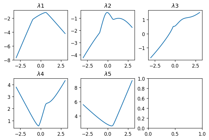
Alright! We see functions having non-trivial shapes. As expected from what we saw in previous posts, the smallest eigenvalue \(\lambda_1\) is concave, the largest \(\lambda_5\) is convex, and all other eigenvalue functions have piecewise-smooth shapes that are neigher convex nor concave. What about \(11\times 11\) matrices?

plot_tridiag_eig_1d(np.random.randn(2, 11), np.random.randn(2, 10))

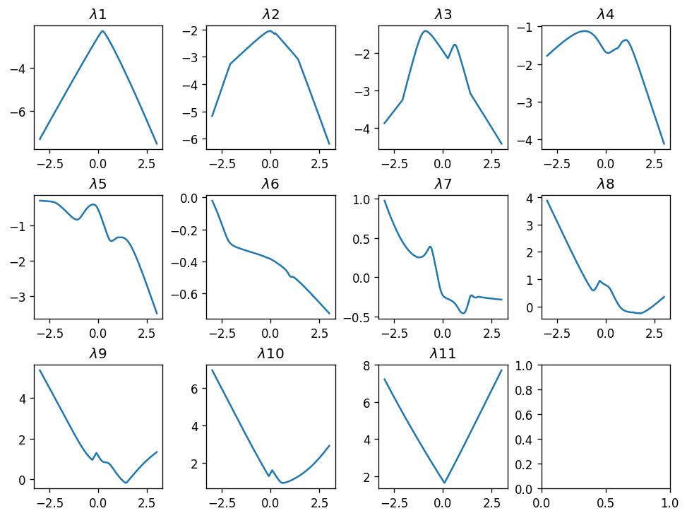
As expected, larger random matrices produce “wilder” shapes - the set of the functions is richer.

Now that we’ve convinced ourselves that tridiagonal matrices have some potential, as a family providing a reasonable balance between speed and expressiveness, let’s move on to a more convincing demonstration of that potential.

Training tridiagonal matrix eigenvalue models

If we want to be able to train with PyTorch, we first need to make sure we can enjoy fast tridiagonal eigenvalue computation there as well. Unfortunately, as of now (PyTorch 2.10), we do not have fast tridiagonal eigenvalue routines in PyTorch, even though tridiagonal and banded matrices do appear in many scientific computing domains. So similarly to a previous post, we will have to implement a custom autograd function that will forward PyTorch tensors to SciPy routines.

As a reminder - we need to subclass torch.autograd.Function and implement two static methods - forward for the computation and backward for the back-propagation of derivatives. This is exactly where we need eigenvectors, and not only the eigenvalues, as we explained in this previous post in the series. As a reminder, for the function \(\lambda_k(\boldsymbol X)\), the “right kind” of generalized derivative is the matrix \(\boldsymbol q_k \boldsymbol q_k^T\), where \(\boldsymbol q_k\) is the corresponding eigenvector. When \(\boldsymbol X\) is tridiagonal, we just need the diagonal and off-diagonal vectors of the \(\boldsymbol q_k \boldsymbol q_k^T\).

So below an autograd function implementing exactly this idea. It appears a bit lengthy, but that’s primarily because it aims to be efficient, and distinguish between two cases: (a) when we need derivatives, e.g., training, and require an eigenvector, and (b) when we do not need derivatives, e.g., inference, and do not require an eigenvector:

import torch

class TridiagEigvalsh(torch.autograd.Function):
    @staticmethod
    def forward(ctx, diag: torch.Tensor, off_diag: torch.Tensor, k: int):
        """Eigenvalue of batch of tridiagonal matrices.

        Args:
            diag (tensor): A M1 x ... x Mn x N tensor representing a batch
                of size M1 x ... x Mn of diagonals of NxN tridiagonal symmetric
                matrices.
            off_diag (tensor): A M1 x ... x Mn x (N - 1) tensor representing
                a batch of size M1 x ... x Mn of off-diagonals of NxN
                tridiagonal symmetric matrices.
            k (int): The eigenvalue index
        """
        need_grad = ctx.needs_input_grad[0] or ctx.needs_input_grad[1]

        diag_np = diag.detach().numpy()
        off_diag_np = off_diag.detach().numpy()
        if need_grad:
            # k-th eigenvalue and eigenvector
            ws_np, Qs_np = sla.eigh_tridiagonal(
                diag_np, off_diag_np, select='i', select_range=(k, k),
                lapack_driver="stemr"
            )
            ws = torch.as_tensor(ws_np, dtype=diag.dtype)
            Qs = torch.as_tensor(Qs_np, dtype=diag.dtype)
            ctx.save_for_backward(Qs.squeeze(-1))
        else:
            # only k-th eigenvalue
            ws_cp = sla.eigvalsh_tridiagonal(
                diag_np, off_diag_np, select='i', select_range=(k, k)
            )
            ws = torch.as_tensor(ws_cp, dtype=diag.dtype)

        return ws.squeeze(-1) # k-th eigenvalue

    @staticmethod
    def backward(ctx, grad_w: torch.Tensor):
        (Qs,) = ctx.saved_tensors  # (..., N) from SciPy

        grad_w = grad_w.to(dtype=Qs.dtype)                 # (...)
        gw = grad_w.unsqueeze(-1)                          # (..., 1)

        grad_diag = gw * Qs.square()                       # (..., N)
        grad_off  = 2 * gw * (Qs[..., :-1] * Qs[..., 1:])  # (..., N-1)

        return grad_diag, grad_off, None

Now let’s try it out. Here is a batch of diagonals of 50 matrices of size 100x100:

diags = torch.randn(50, 100)
off_diags = torch.randn(50, 99)

Now let’s try applying our PyTorch function to the raw tensors. Note - they do not require a gradient, since they aren’t trainable parameters, so we’re going through the no_grad path:

%%timeit -r 30 -n 100
w = TridiagEigvalsh.apply(diags, off_diags, 2).sum()

3.71 ms ± 91.7 µs per loop (mean ± std. dev. of 30 runs, 100 loops each)

Whoa! That’s fast! Now let’s try doing it with trainable parameters:

diags_param = torch.nn.Parameter(diags)
off_diags_param = torch.nn.Parameter(off_diags)

%%timeit -r 30 -n 100
w = TridiagEigvalsh.apply(diags_param, off_diags_param, 2).sum()
w.backward()

4.88 ms ± 205 µs per loop (mean ± std. dev. of 30 runs, 100 loops each)

Pretty fast - a mini-batch of 50 tridiagonal matrices of size 100x100 can compute gradients in approximately 5 milliseconds. Comparing it with approximately 35 milliseconds for full dense matrices - quite a speedup. For convenience, let’s wrap our autograd function class with a simple Python function:

def tridiag_eigvalsh(
        diag: torch.Tensor, off_diag: torch.Tensor, k: int
    ) -> torch.Tensor:
    return TridiagEigvalsh.apply(diag, off_diag, k)

So now, to train a model we need a torch module representing our \(f(\boldsymbol x, \boldsymbol A_{0..n})\) for the tri-diagonal case. This means our trainable parameters are the diagonals and the off-diagonals of the matrices \(\boldsymbol A_0, \dots, \boldsymbol A_n\). Note that both the diagonal vector and the off-diagonal vector of \(\mathcal{A}(\boldsymbol x)\) are just linear functions of \(\boldsymbol x\), so we can express them as simple torch.nn.Linear layers. This yields an almost magically simple class:

from torch import nn

class TridiagSpectral(nn.Module):
    def __init__(self, *, num_features: int, dim: int, eig_idx: int):
        super().__init__()
        self.eig_idx = eig_idx
        self.diag = nn.Linear(num_features, dim)
        self.off_diag = nn.Linear(num_features, dim - 1)

    def forward(self, x):
        return tridiag_eigvalsh(self.diag(x), self.off_diag(x), self.eig_idx)

Now we can use it for training, like any PyTorch model. So let’s try learning a classifier that detects whether we have either two or five ones in a vector:

def toy_function(x: torch.Tensor):
    return torch.maximum(
        x.sum(axis=-1) == 2,
        x.sum(axis=-1) == 5
    ).to(dtype=torch.float32)

Now we shall apply it to learning this function over 12-dimensional vectors. So let’s generate all binary vectors and compute their true label:

n_features = 12
X = torch.cartesian_prod(*([torch.tensor([0., 1.])] * n_features)) 
y = toy_function(X)

This set should contain \(2^12 = 4096\) vectors. And before training, let’s divide the features and labels into a train and evaluation set:

torch.manual_seed(42)
train_mask = torch.rand(len(X)) < 0.5
X_train = X[train_mask, :]
y_train = y[train_mask]
X_test = X[~train_mask, :]
y_test = y[~train_mask]

Alright! We’re ready to train a classifier on (X_train, y_train) and evaluate it on (X_test, y_test). This would be a good time to introduce the fitstream library, which is very convenient for training PyTorch models on small in-memory datasets. Recall that we found it very convenient to hide the training loop behind a Python generator that yields an event on every epoch. So this is what this library does - it performs a pretty standard PyTorch training loop, and yields a dict with some data at the end of each epoch. Let’s first install it in our notebook:

%pip install -q fitstream

Now let’s use it. Below is a short snippet demonstrating how we iterate over the first 3 events, which are simple Python dicts, and use Python’s pprint library to nicely print each dict:

import fitstream as fts
from pprint import pprint

# define model and optimizer
dim = 3
model = TridiagSpectral(num_features=n_features, dim=dim, eig_idx=dim // 2)
optim = torch.optim.Adam(model.parameters(), lr=1e-1)

# use FitStream to obtain the event generator
events = fts.epoch_stream(
    (X_train, y_train), model, optim, nn.BCEWithLogitsLoss(), batch_size=32
)

# iterate over the first three events
for _, event in zip(range(3), events):
    pprint(event)
    print('---')

{'model': TridiagSpectral(
  (diag): Linear(in_features=12, out_features=3, bias=True)
  (off_diag): Linear(in_features=12, out_features=2, bias=True)
),
 'step': 1,
 'train_loss': 0.47607117891311646,
 'train_time_sec': 0.19717628799844533}
---
{'model': TridiagSpectral(
  (diag): Linear(in_features=12, out_features=3, bias=True)
  (off_diag): Linear(in_features=12, out_features=2, bias=True)
),
 'step': 2,
 'train_loss': 0.4695621430873871,
 'train_time_sec': 0.17527212999993935}
---
{'model': TridiagSpectral(
  (diag): Linear(in_features=12, out_features=3, bias=True)
  (off_diag): Linear(in_features=12, out_features=2, bias=True)
),
 'step': 3,
 'train_loss': 0.46067821979522705,
 'train_time_sec': 0.1757020229997579}
---

Now we see what we get - each dict contains our model, the epoch index in the step key, the training loss, and the training time in seconds. Pretty minimal, so the library comes with some helper functions to take this minimal event stream, and enrich it.

It has the pipe function, which lets us pipe the event stream through a sequence of transformations. So let’s introduce the first transformation - take, which simply takes the head of the event stream of the specified size. For example, this will produce 5 events:

# define model and optimizer
dim = 3
model = TridiagSpectral(num_features=n_features, dim=dim, eig_idx=dim // 2)
optim = torch.optim.Adam(model.parameters(), lr=1e-1)

# pipe the epoch stream through the "take" transformation
events = fts.pipe(
    fts.epoch_stream(
        (X_train, y_train), model, optim, nn.BCEWithLogitsLoss(), batch_size=32
    ),
    fts.take(5)
)

for event in events:
    print(event['step'], event['train_loss'])

1 0.4920884072780609
2 0.46535375714302063
3 0.4354994297027588
4 0.4041599929332733
5 0.32225537300109863

The second important transformation is augment, which adds additional keys to each event. Here is an example of adding a key with the training loss squared:

# define model and optimizer
dim = 3
model = TridiagSpectral(num_features=n_features, dim=dim, eig_idx=dim // 2)
optim = torch.optim.Adam(model.parameters(), lr=1e-1)

# pipe the epoch stream through the "take" transformation
events = fts.pipe(
    fts.epoch_stream(
        (X_train, y_train), model, optim, nn.BCEWithLogitsLoss(), batch_size=32
    ),
    fts.augment(lambda event: {"loss_squared": event["train_loss"] ** 2}),
    fts.take(5)
)

for event in events:
    print(event['step'], event["train_loss"], event['loss_squared'])

1 0.4896900951862335 0.23979638932350245
2 0.45949652791023254 0.21113705916155912
3 0.46307340264320374 0.2144369762355547
4 0.44300273060798645 0.19625141932613221
5 0.4168809950351715 0.1737897640215147

Now, this is all nice, but the library is richer. It comes with augmentations for adding a validation loss, early stopping, or simply executing a function on every event. So here is a generator of events for a full-fledged training procedure with a validation loss and early stopping that also prints the losses every 10 epochs:

dim = 3
model = TridiagSpectral(num_features=n_features, dim=dim, eig_idx=dim // 2)
optim = torch.optim.Adam(model.parameters(), lr=1e-1)
events = fts.pipe(
    fts.epoch_stream(
        (X_train, y_train), model, optim, nn.BCEWithLogitsLoss(), batch_size=64
    ),
    fts.augment(fts.validation_loss((X_test, y_test), nn.BCEWithLogitsLoss())),
    fts.early_stop(key="val_loss", patience=5),
    fts.tap(fts.print_keys("train_loss", "val_loss"), every=10),
    fts.take(100)
)

Finally, the library comes with a set of collector functions that iterate over the events and collect them into various data structures. Here it will be convenient to use collect_pd, which collects the event dicts into a Pandas DataFrame. So here is an example of collecting the above event stream into a data frame, and then plotting the training and validation losses:

training_log = fts.collect_pd(events)
training_log.plot(x="step", y=["train_loss", "val_loss"], title='Dim = 3')

step=0001 train_loss=0.4908 val_loss=0.4681
step=0011 train_loss=0.3369 val_loss=0.3147
step=0021 train_loss=0.1540 val_loss=0.1516
step=0031 train_loss=0.0768 val_loss=0.0926
step=0041 train_loss=0.0500 val_loss=0.0725
step=0051 train_loss=0.0363 val_loss=0.0621
step=0061 train_loss=0.0291 val_loss=0.0580
step=0071 train_loss=0.0241 val_loss=0.0557
step=0081 train_loss=0.0210 val_loss=0.0538
step=0091 train_loss=0.0186 val_loss=0.0536
step=0101 train_loss=0.0172 val_loss=0.0539

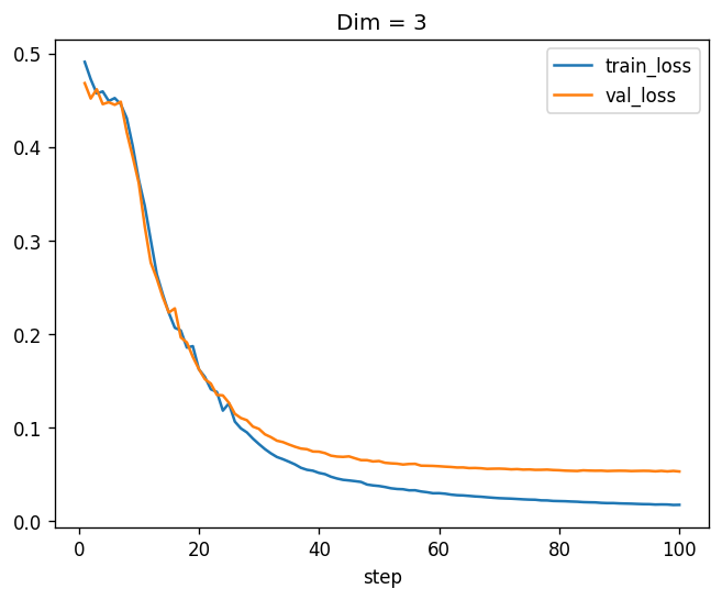
Nice! We see that the model is learning, which is encouraging. Before we do more experiments, let’s write a function that will construct such a training procedure for us and collect the events to a dataframe:

def run_experiment_bce(model, lr=1e-1, batch_size=64, max_epochs=100):
    optim = torch.optim.Adam(model.parameters(), lr=lr)
    events = fts.pipe(
        fts.epoch_stream(
            (X_train, y_train), model, optim, nn.BCEWithLogitsLoss(), batch_size=batch_size
        ),
        fts.augment(fts.validation_loss((X_test, y_test), nn.BCEWithLogitsLoss())),
        fts.early_stop(key="val_loss", patience=5),
        fts.take(max_epochs)
    )
    return fts.collect_pd(events)

Now we can easily plot similar losses for \(5 \times 5\) tridiagonal matrices:

training_log_5 = run_experiment_bce(
    TridiagSpectral(num_features=n_features, dim=5, eig_idx=2)
)
training_log_5.plot(x="step", y=["train_loss", "val_loss"], title='Dim = 5')

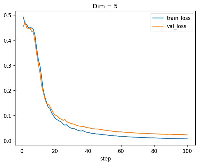
Much better! Now the validation loss is very close to zero as well. Now let’s move to \(9 \times 9\) matrices:

training_log_9 = run_experiment_bce(
    TridiagSpectral(num_features=n_features, dim=9, eig_idx=4)
)
training_log_9.plot(x="step", y=["train_loss", "val_loss"], title='Dim = 9')

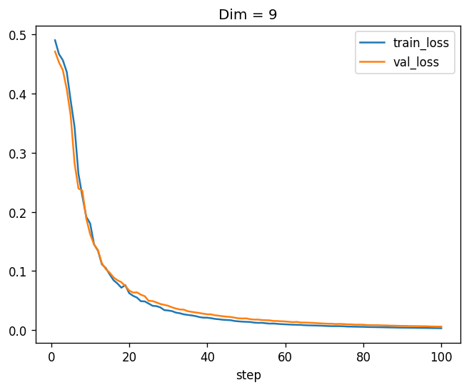
Beautiful! Apparently, a model with \(9 \times 9\) tridiagonal symmetric matrices, which has \(13 \times (9 + 8) = 221\) parameters, can learn this function from data almost perfectly. And conceptually, this is just a linear function of the features followed by a non-linear function - the matrix eigenvalue. Just one neuron! You can try it, but a “classical” neuron cannot learn this function.

So now that we’re convinced that the machinery is working, let’s try it on the dataset that accompanies this series - the California Housing dataset we have built into our Colab notebooks.

California housing training

Recall that the dataset is about predicting housing prices in California based on some features. I will skip the part where we read the data, normalize features and targets, and split the data into training and test sets. We’ve already done it in previous posts in this series, and the notebook contains the full code. So here we’ll assume our training data is in X_train, y_train, our evaluation set is X_test, y_test, and the number of features is in num_features. Moreover, since our labels are scaled, we also have label_scale, which is the factor that transforms the training / eval RMSE back to the original units in the dataset - dollars.

First, let’s define a simple function that computes the RMSE in dollars:

def scaled_rmse(y_true, y_pred):
    mse = nn.functional.mse_loss(y_pred, y_true)
    return torch.sqrt(mse) * label_scale

Now, we can define a full-fledged training procedure with the FitStream library we just introduced. When experimenting, I noticed that learning rate scheduling improves convergence substantially and I can work with less epochs, so I also used a learning rate scheduler with warmup - just like we do with LLMs. It first increases the learning rate for a few epochs (warmup), and then decreases it slowly towards zero (cooldown). It is implemented in the OneCycleLR class from PyTorch. So here is our full training procedure:

from torch.optim.lr_scheduler import OneCycleLR

def complete_training_stream(
        dim, n_epochs, warmup_fraction=0.1, lr=5e-3, batch_size=64,
    ):
    model = TridiagSpectral(num_features=num_features, dim=dim, eig_idx=dim // 2)
    optim = torch.optim.Adam(model.parameters(), lr=lr)
    sched = OneCycleLR(
        optim, max_lr=lr, total_steps=n_epochs, pct_start=warmup_fraction, anneal_strategy='linear'
    )

    epoch_events = fts.epoch_stream((X_train, y_train), model, optim, nn.MSELoss(), batch_size=batch_size)
    return fts.pipe(
        epoch_events,
        fts.take(n_epochs),
        fts.augment(fts.validation_loss((X_test, y_test), scaled_rmse)), # <-- here we use scaled_rmse
        fts.augment(lambda event: {"lr": optim.param_groups[0]['lr']}),
        fts.early_stop(key="val_loss", patience=n_epochs // 10),
        fts.tick(sched.step),
    )

Note where we use our scaled_rmse - it is inserted as the validation loss to the stream. Now, let’s try it out with 11-dimensional matrices for 20 epochs:

training_log = fts.collect_pd(complete_training_stream(11, 20))
print(training_log)

This is what I got:

step  train_loss  train_time_sec       val_loss        lr
0      1    0.893857        1.095248  101073.101562  0.000200
1      2    0.404809        1.114020   65408.109375  0.005000
2      3    0.298268        1.138942   62557.234375  0.004722
3      4    0.277326        1.107545   61244.425781  0.004444
4      5    0.268057        1.099500   60413.164062  0.004167
5      6    0.262378        1.105777   59918.421875  0.003889
6      7    0.256854        1.100250   59919.507812  0.003611
7      8    0.253308        1.095398   59363.906250  0.003333
8      9    0.250837        1.091576   59104.089844  0.003056
9     10    0.248961        1.083466   59065.980469  0.002778
10    11    0.246233        1.092109   58896.339844  0.002500
11    12    0.244495        1.114625   58766.113281  0.002222
12    13    0.241918        1.118336   58610.593750  0.001944
13    14    0.240912        1.101395   58488.941406  0.001667
14    15    0.239700        1.100444   58310.894531  0.001389
15    16    0.238621        1.096240   58618.683594  0.001111
16    17    0.237742        1.085707   58579.175781  0.000833

We can see the model is training, the learning rate increased in the first two epochs, as expected, since 10% of the epochs are warmup. It stopped after 17 epochs due to the early stopping mechanism whose patience is two epochs (again, 10% of the maximum).

We can also write a nice function for plotting the learning rate and the validation loss. It’s a bit of boilerplate, for using the primary y-axis for the validation loss, and the secondary y-axis for the learning rate.

def plot_log(log, title=None):
    fig, ax = plt.subplots()

    ax.plot(log.step, log.val_loss, color='blue',
            label=f'RMSE (best=${log.val_loss.min():.2f})')
    ax.set_ylabel("Error ($)")
    ax.grid()

    lr_ax = ax.twinx()
    lr_ax.plot(log.step, log.lr, label='Learning rate',
               color='gray', linestyle='dotted', linewidth=1)
    lr_ax.set_ylabel("Learning rate")

    ax.legend()
    if title is not None:
        ax.set_title(title)
    fig.show()

plot_log(training_log)

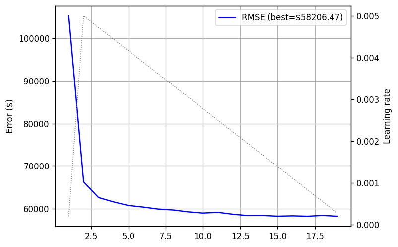
In blue we see the validation loss, whereas in dotted black we see the learning rate. We can nicely see the warmup and cooldown stages.

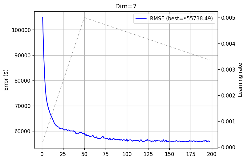
Alright, so now that we have all the machinery in place, let’s try training some model with more epochs. I used 500 epochs in all the experiments, which was enough to train both smaller and larger models. So let’s try 7-dimensional tridiagonal matrices:

training_log_7 = fts.collect_pd(complete_training_stream(7, 500))
plot_log(training_log_7, title='Dim=7')

How about 11-dimensional tridiagonals?

training_log_11 = fts.collect_pd(complete_training_stream(11, 500))
plot_log(training_log_11, title='Dim=11')

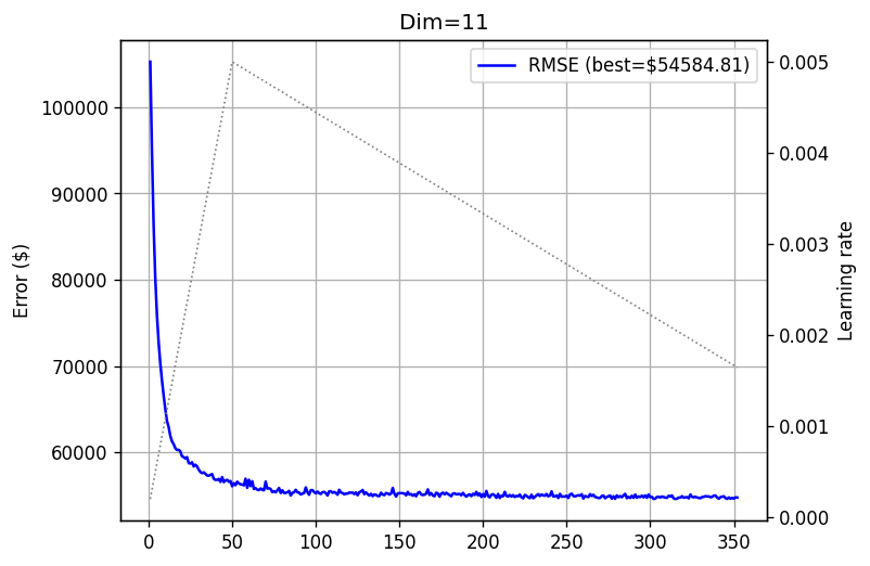
Nice! Increasing matrix size reduces the error, meaning that performance scales with model size. But remember - it is just one neuron! How about \(15 \times 15\) matrices?

training_log_15 = fts.collect_pd(complete_training_stream(15, 500))
plot_log(training_log_15, title='Dim=15')

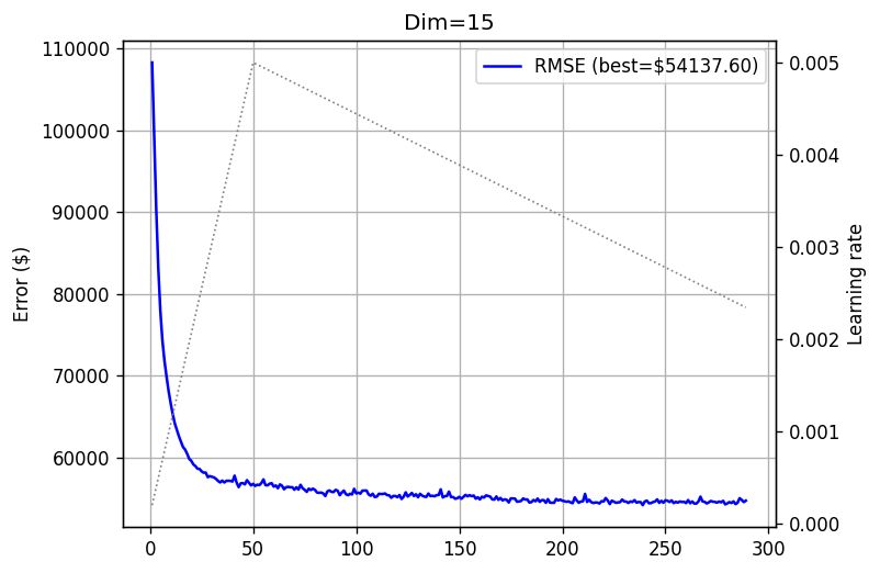
Another slight improvement. What about \(45 \times 45\) matrices?

training_log_45 = fts.collect_pd(tqdm(complete_training_stream(45, 500)))
plot_log(training_log_45, title='Dim=45')

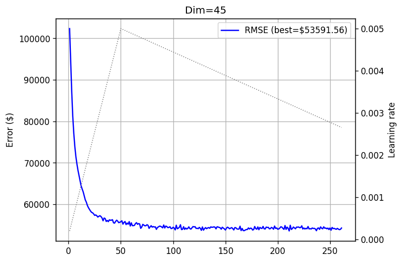
I can share, and you can see it by running the notebook yourself, that each such experiment takes 3-4 minutes. Just to get a feeling - compared to dense matrix experiments we conducted in previous posts, this is much faster, and without any GPU. I’m pretty sure that if PyTorch had tridiagonal support, we could have run each experiment in seconds. But unfortunately - it does not.

Comparing it to dense experiments we conducted with the same dataset and similar matrix sizes in this post, which took us 31 minutes on an NVidia L4 GPU for a \(45 \times 45\) matrix, while achieving a similar test error - we clearly see the difference. No GPU, an order of magnitude faster, and a similar performance at least on this dataset.

Of course - the above are not proper experiments I’d include in a paper. I haven’t conducted any hyperparameter search, perhaps a different optimizer could be better, etc…, but we see the point.

Summary

To summarize, we can see that restricting ourselves to eigenvalue model families where all matrices are simultaneously tri-diagonalizable can be useful to strike a good balance between speed and expressiveness. Let us recall why this model family is interesting - it’s just one neuron, a linear (matrix) function composed with a non-linearity, that is quite expressive, while being fairly interpretable. These nice properties haven’t gone anywhere - spectral norms of our tridiagonal matrices are still a reasonable way to think of importance, and provide a certificate for sensitivity of the model to changes in that feature.

We do, however, see slow convergence. 500 epochs is quite a lot, and even though our training procedure stops beforehand due to the early stopping mechanism, it’s still a few hundred epochs. Even if I throw the best practices at it, such as learning rate scheduling, early stopping, and others - it’s still quite slow. At this stage, this is a price we pay for having a model that is, on the one hand, just one fairly interpretable neuron, but on the other hand can be improved by scaling.

We have many more questions to explore in this series. For example - can we prune any dense eigenvalue model to tridiagonal form? Can we make it converge faster? How do we stack such models as layers of a larger neural network? Stay tuned!