“Proximal Point to the Extreme - Factorization Machines"
This post is part of the series "Proximal point", and is not self-contained.
Series posts:
-
“Proximal Point - warmup"
-
“Proximal point - convex on linear losses"
-
“Proximal Point - regularized convex on linear I"
-
“Proximal Point - regularized convex on linear II"
-
“Proximal Point is, after all, yet another gradient method"
-
“Selective approximation - the prox-linear method for training arbitrary models"
-
“Proximal Point with Mini Batches"
-
“Proximal Point with Mini Batches - Convex On Linear"
-
“Proximal Point with Mini Batches - Regularized Convex On Linear"
- “Proximal Point to the Extreme - Factorization Machines" (this post)
- “Proximal Point - warmup"
- “Proximal point - convex on linear losses"
- “Proximal Point - regularized convex on linear I"
- “Proximal Point - regularized convex on linear II"
- “Proximal Point is, after all, yet another gradient method"
- “Selective approximation - the prox-linear method for training arbitrary models"
- “Proximal Point with Mini Batches"
- “Proximal Point with Mini Batches - Convex On Linear"
- “Proximal Point with Mini Batches - Regularized Convex On Linear"
- “Proximal Point to the Extreme - Factorization Machines" (this post)
Intro
In this final episode of the proximal point series I would like to take the method to the extreme, and show that we can actually train a model which composed with an appropriate loss produces functions which are non-linear and non-convex: we’ll be training a factorization machine for classification problems without linearly approximating loss functions and relying on loss gradients. Factorization machines and variants are widely used in recommender systems, i.e. recommending movies to users. I assume readers are familiar with the basics, and below I provide only a brief introduction, so that throughout this post we have a consistent notation and terminology, and understand the assumptions we make.
I do not claim that it is the best method for training factorization machines, but it is indeed an interesting challenge in order to see what are the limits of efficiently implementable proximal point methods. We’ll have some more advanced optimization theory, even some advanced linear algebra, but most importantly, at the end of the journey we’ll have a github repo with code which you can run and try it out on your own dataset!
Since it’s an ‘academic’ experiment in nature, and I do not aim to implement the most efficient and robust code, we’ll make some simplifying assumptions. However, a production-ready training algortithm will not be far away from the implementation we construct in this post.
A quick intro
Let’s begin by a quick introduction to factorization machines. Factorization machines are usually trained on categorical data representing the users and the items, for example, age group and gender may be user features, while product category and price group may be item features. The model embeds each categorical feature to a latent space of some pre-defined dimension \(k\), and the model’s prediction comprises of inner products of the latent vectors corresponding to the current samples. The most simple variant are second order factorization machines, which we the focus of this post.
Formally, our second-order factorization machine \(\sigma(w, x)\) is given a binary input \(w \in \{0, 1\}^m\) which is a one-hot encoding of a subset of at most \(m\) categorical features. For exampe, suppose we would like to predict the affinity of people with chocolate. Assume, for simplicity, that we have only two user gender values \(\{ \mathrm{male}, \mathrm{female} \}\), and two two age groups \(\{ \mathrm{young}, \mathrm{old} \}\). For our items, suppose we have only one feature - the chocolate type, which may take the values \(\{\mathrm{dark}, \mathrm{milk}, \mathrm{white}\}\). In that case, the model’s input is the vector of zeros and ones encoding feature indicators:
\[w=(w_{\mathrm{male}}, w_{\mathrm{female}}, w_{\mathrm{young}}, w_{\mathrm{old}}, w_{\mathrm{dark}}, w_{\mathrm{milk}}, w_{\mathrm{white}}).\]A young male who tasted dark chocolate is represented by the vector
\[w = (1, 0, 1, 0, 1, 0, 0).\]In general, the vector \(w\) can be defined by arbitrary real numbers, but I promised that we’ll make simplifying assumptions :)
The model’s parameter vector \(x = (b_0, b_1, \dots, b_m, v_1, \dots, v_m)\) is composed of the model’s global bias \(b_0 \in \mathbb{R}\), the biases \(b_i \in \mathbb{R}\) for the features \(i\in \{1, \dots, m\}\), and the latent vectors \(v_i \in \mathbb{R}^k\) for the same features with \(k\) being the embeddig dimension. The model computes:
\[\sigma(w, x) := b_0 + \sum_{i = 1}^m w_i b_i + \sum_{i = 1}^m\sum_{j = i + 1}^{m} (v_i^T v_j) w_i w_j.\]Let’s set up some notation which will become useful throughout this post. We will detote a set of consecutive integers by \(i..j=\{i, i+1, \dots, j\}\), and the set of distinct pairs of the integers \(J\) is denoted by \(P[J]=\{ (i,j) \in J\times J : i<j \}\). Consequently, we can re-write:
\[\sigma(w,x)=b_0 + \sum_{i\in 1..m} w_i b_i+\sum_{(i,j) \in P[1..m]} (v_i^T v_j) w_i w_j\]At this stage this notation does not seem useful, but it will simplify things later in this post. We’ll use this notation consistently throughout the post.
For completeness, let’s implement a factorization machine in PyTorch. To that end, recall a famous trick introduced by Steffen Rendle in his pioneering paper1 on factorization machines, based on the formula
\[\Bigl\| \sum_{i\in 1..m} w_i v_i \Bigr\|_2^2 = \sum_{i\in 1..m} \|w_i v_i\|_2^2 + 2 \sum_{(i,j)\in P[1..m]} (v_i^T v_j) w_i w_j.\]After re-arrangement, the above results in:
\[\sum_{(i,j)\in P[1..m]} (v_i^T v_j) w_i w_j= \frac{1}{2}\Bigl\| \sum_{i\in1.m} w_i v_i \Bigr\|_2^2-\frac{1}{2}\sum_{i\in1..m} \|w_i v_i\|_2^2. \tag{L}\]Since \(w\) is a binary vector, we can associate it with its non-zero indices \(\operatorname{nz}(w)\), and the right-hand side of above term can be written as:
\[\frac{1}{2}\Bigl\| \sum_{i \in \operatorname{nz}(w)} v_i \Bigr\|_2^2-\frac{1}{2}\sum_{i \in \operatorname{nz}(w)} \| v_i\|_2^2.\]Consequently, the pairwise terms can be computed in time linear in the number of non-zero indicators in \(w\), instead of the quadratic time imposed by the naive way. The PyTorch implementation below uses the trick above.
import torch
from torch import nn


class FM(torch.nn.Module):
    def __init__(self, m, k):
        super(FM, self).__init__()

        self.bias = nn.Parameter(torch.zeros(1))
        self.biases = nn.Parameter(torch.zeros(m))
        self.vs = nn.Embedding(m, k)

        with torch.no_grad():
            torch.nn.init.normal_(self.vs.weight, std=0.01)
            torch.nn.init.normal_(self.biases, std=0.01)

    def forward(self, w_nz):  # since w are indicators, we simply use the non-zero indices
        vs = self.vs(w_nz)
        # in vs:
        #   dim = 0 is the mini-batch dimension. We would like to operate on each elem. of a mini-batch separately.
        #   dim = 1 are the embedding vectors
        #   dim = 2 are their components.

        pow_of_sum = vs.sum(dim=1).square().sum(dim=1)  # sum vectors -> square -> sum components
        sum_of_pow = vs.square().sum(dim=[1,2])         # square -> sum vectors and components
        pairwise = 0.5 * (pow_of_sum - sum_of_pow)

        biases = self.biases
        linear = biases[w_nz].sum(dim=1)                # sum biases for each element of the mini-batch

        return pairwise + linear + self.bias
If we are interested in solving a regression problem, i.e. predicting arbitrary real values, such as a score a person would give to the chocolate, we can use \(\sigma\) directly to make predictions. If we are in the binary classification setup, i.e. predict the probability that a person likes the corresponding chocolate, we compose \(\sigma\) with a sigmoid, and predict \(p(w,x) = (1+e^{-\sigma(w,x)})^{-1}\).
The setup
In this post we are interested in the binary classification setup, with the binary cross-entropy loss. Namely, given a label \(y \in \{0,1\}\) the loss is:
\[-y \ln(p(w,x)) - (1 - y) \ln(1 - p(w,x)).\]For example, if we would like to predict which chocolate people like, we could train the model on a data-set with samples of people who liked a certain chocolate having the label \(y = 1\), and people who tasted but did not like it will have the lable \(y = 0\). Having trained the model, we can recommend chocolate to a person by choosing the one with the highest probability of being liked.
Using a simple transformation \(\hat{y} = 2y-1\) we can remap the labels to be in \(\{-1, 1\}\) instead. Then, it isn’t hard to verify that the binary cross-entropy loss above reduces to:
\[\ln(1+\exp(-\hat{y} \sigma(w,x))).\]Consequently, our aim will be training over the set \(\{ (w_i, \hat{y}_i) \}_{i=1}^n\) by minimizing the average loss
\[\frac{1}{n} \sum_{i=1}^n \underbrace{\ln(1+\exp(-\hat{y}_i \sigma(w_i, x)))}_{f_i(x)}.\]Instead of using regular SGD-based methods for training, which construct a linear approximations of \(f_i\) and are able to use only the information provided by the gradient, we will avoid approximating and use the loss itself via the stochastic proximal point algorithm - at iteration \(t\) choose \(f \in \{f_1, \dots, f_n\}\) and compute:
\[x_{t+1} = \operatorname*{argmin}_x \left\{ f(x) + \frac{1}{2\eta} \|x - x_t\|_2^2 \right\}. \tag{P}\]Careful readers might notice that the formula above is total nonsense in general. Why? Well, the each \(f\) is a non-convex function of \(x\). If \(f\) was convex, we would obtain a unique and well-defined minimizer \(x_{t+1}\). However, in general, the \(\operatorname{argmin}\) above is a set of minimizers, which might even be empty! In this post we will attempt to mitigate this issue:
- Discover the conditions on the step-size \(\eta\) which ensure that we have a unique minimizer \(x_{t+1}\).
- Find an explicit formula, or a simple algorithm, for computing \(x_{t+1}\).
Having done the above, we’ll be able to construct an algorithm which can train classifying factorization machines which exploit the exact loss function, instead of just relying on its slope as in SGD.
Duality strikes again
In previous posts we heavily relied on duality in general, and convex conjugates in particular, and this post is no exception. Recall, that the convex conjugate of the function \(h\) is defined by:
\[h^*(z) = \sup_x \{ x^T z - h(x) \},\]and recall also that in a previous post we saw that \(h(t)=\ln(1+\exp(t))\) is convex, and its convex conjugate is:
\[h^*(z) = \begin{cases} z\ln(z) + (1 - z) \ln(1 - z), & 0 < z < 1 \\ 0, & \text{otherwise}. \end{cases}\]An interesting result about conjugates is that under some technical conditions, which hold for \(h(t)\) above, we have \(h^{**} = h\), namely, the conjugate of \(h^*\) is \(h\). Moreover, in our case the \(\sup\) in the conjugate’s definition can be replaced with a \(\max\), since the supermum is always attained2. Why is it useful? Since now we know that:
\[\ln(1+\exp(t))=\max_z \left\{ t z - z \ln(z) - (1-z) \ln(1-z) \right\}.\]Consequently, the term inside the \(\operatorname{argmin}\) of the proximal point step (P) can be written as:
\[\begin{aligned} f(x) &+ \frac{1}{2\eta} \|x - x_t\|_2^2 \\ &\equiv \ln(1+\exp(-\hat{y} \sigma(w,x))) + \frac{1}{2\eta} \|x - x_t\|_2^2 \\ &= \max_z \Bigl\{ \underbrace{ -z \hat{y} \sigma(w,x) + \frac{1}{2\eta} \|x - x_t\|_2^2 - z\ln(z) - (1-z)\ln(1-z) }_{\phi(x,z)} \Bigr\}. \end{aligned}\]Since we are interested in minimizing the above, we will be solving the saddle-point problem:
\[\min_x \max_z \phi(x,z). \tag{Q}\]Convex duality theory has another interesting form - it provides conditions on saddle-point problems which ensure that we can switch the order of \(\min\) and \(\max\) to obtain an equivalent problem. Why is it interesting? Because switching the order produces
\[\max_z \underbrace{ \min_x \phi(x,z)}_{q(z)},\]and finding the optimal \(z\) means maximizing the one dimensional function \(q\), which may even be as simple as a high-school calculus exercise.
So here is relevant duality theorem, which is a simplification of Sion’s minimax theorem from 1958 for this post:
Let \(\phi(x,z)\) be a continuous function which is convex in \(x\) and concave in \(z\). Suppose that the domain of \(\phi\) over \(z\) is compact, i.e. a closed a bounded set. Then,
\[\min_x \max_z \phi(x,z) = \max_z \min_x \phi(x,z)\]
In our case, it’s easy to see that \(\phi\) is indeed concave in \(z\) using negativity of its second derivative, and its domain, the interval \([0,1]\), is indeed compact. What we require for the theorem’s conditions to hold is convexity in \(x\), which is what we explore next. Then, we’ll see that \(q\), despite not being so simple, can still be quite efficiently maximized. The theorem does not imply that a pair \((x, z)\) solving the max-min problem also solves the min-max problem, but in our case the max-min problem has a unique solution, and in that particular case it indeed also solves the min-max problem.
Consequently, having found \(z^*=\operatorname{argmax}_z q(z)\), we by construction obtain a formula for computing the optimal \(x\): \(x_{t+1} = \operatorname*{argmin}_x ~ \phi(x, z^*).\)
So let’s begin by ensuring that the conditions for Sion’s theorem hold. Ignoring the terms of \(\phi\) which do not depend on \(x\), we need to study the convexity of the following part as a function of \(x\):
\[(*) = -z \hat{y} \sigma(w,x) + \frac{1}{2\eta} \|x - x_t\|_2^2.\]To that end, we need to open the ‘black box’ and look inside \(\sigma\) again. That’s going to be a bit technical, but it gets us where we need. If you don’t wish to read all the details, you may skip to the conclusion below.
Recall, the composition \(x = (b_0, b_1, \dots, b_m, v_1, \dots, v_m)\) and the definition
\[\sigma(w, b_0, \dots, b_m, v_1, \dots, v_m) = b_0 + \sum_{i\in1..m} w_i b_i + \sum_{(i,j)\in P[1..m]} (v_i^T v_j) w_i w_j.\]Consequently, we can re-write \((*)\) as:
\[\begin{aligned} (*) =& \color{blue}{-z \hat{y} \Bigl[ b_0 + \sum_{i\in1..m} w_i b_i \Bigr] + \frac{1}{2\eta} \|b - b_t\|_2^2} \\ & \color{brown}{- z \hat{y} \sum_{i\in P[1..m]} (v_i^T v_j) w_i w_j + \frac{1}{2\eta} \sum_{i\in1..m} \| v_i - v_{i,t} \|_2^2}. \end{aligned}\]The part colored in blue is always convex - it is the sum of a linear function and a convex-quadratic one. It remains to study the convexity of the brown part. Re-arranging the formula for \(\|v_i + v_j\|_2^2\), we obtain that:
\[v_i^T v_j = \frac{1}{2} \|v_i + v_j\|_2^2 - \frac{1}{2}\|v_i\|_2^2 - \frac{1}{2} \|v_j\|_2^2.\]Denoting \(\alpha_{ij} = -z \hat{y} w_i w_j\) we can re-write the brown part as: \(\begin{aligned} \color{brown}{\text{brown}} &= \sum_{i\in P[1..m]} |\alpha_{ij}| v_i^T ( \operatorname{sign}(\alpha_{ij}) v_j) + \frac{1}{2\eta} \sum_{i\in1..m} \| v_i - v_{i,t} \|_2^2 \\ &= \frac{1}{2}\sum_{i\in P[1..m]} |\alpha_{ij}| \left[ \|v_i + \operatorname{sign}(\alpha_{ij}) v_j\|_2^2 - \|v_i\|_2^2-\|v_j\|_2^2 \right] + \sum_{i\in1..m} \left[ \| v_i \|_2^2 \color{darkgray}{- 2 v_i^T v_{i,t} + \|v_{i,t}\|_2^2} \right] \end{aligned}\)
The grayed-out part on the right is linear in \(v_i\), so it’s convex. Since \(\alpha_{ij} = \alpha_{ji}\), to simplify notation we define \(\alpha_{ii}=0\), and the remaining non-greyed parts can be written as:
\[\frac{1}{2} \sum_{i\in P[1..m]} |\alpha_{ij}| \|v_i + \operatorname{sign}(\alpha_{ij}) v_j\|_2^2 + \sum_{i\in 1..m} \left(\frac{1}{2\eta} - \sum_{j\in 1..m} |\alpha_{ij}|\right) \|v_i\|_2^2.\]Again, the first sum is a sum of convex-quadratic functions, and thus convex. For the second part to be convex, we require that for each \(i\) we have
\[\frac{1}{2\eta} \geq \sum_{j\in 1..m} |\alpha_{ij}|,\]or equivalently that the step-size \(\eta\) must satisfy
\[\eta \leq \frac{1}{2\sum_{j \in 1..m} |\alpha_{ij}|}\]Since \(\vert \alpha_{ij} \vert \leq 1\), we can easily deduce that for any step-size \(\eta \leq \frac{1}{2m}\), we obtain a convex \(\phi\). A better bound is obtained if we have a bound on the number of indicators in the vector \(w\) which may be non-zero at the same time. For example, if we have six categorical fields, we will have at most six non-zero elements in \(w\), and thus \(\eta \leq \frac{1}{12}\).
Convexity is nice if we want Sion’s theorem to hold, but if we want a unique minimizer \(x_{t+1}\) we need strict convexity, which is obtained by using a strict inequality - replace \(\leq\) with \(<\). In this post we will assume that we have at most \(d\) categorical features, and use step-sizes which satisfy
\[\eta \leq \frac{1}{2d+1} < \frac{1}{2d}.\]Computing \(x_{t+1}\)
Suppose that Sion’s theorem holds, and that we can obtain a unique minimizer \(x_{t+1}\). How do we compute it? Well, Sion’s theorem lets us switch the order of \(\min\) and \(\max\), so we are aiming to solve:
\[\max_z \underbrace{ \min_x \phi(x,z)}_{q(z)},\]and explicitly writing \(\phi\) we have:
\[\begin{aligned} q(z) = \min_{b,v_i} \Bigl\{ &-z \hat{y} \Bigl[ b_0 + \sum_{i\in 1..m} w_i b_i \Bigr] + \frac{1}{2\eta} \|b - b_t\|_2^2 \\ &- z \hat{y} \sum_{(i,j) \in P[1..m]} (v_i^T v_j) w_i w_j + \frac{1}{2\eta} \sum_{i\in 1..m} \| v_i - v_{i,t} \|_2^2 \\ &- z \ln(z) - (1-z) \ln(1-z) \Bigr\} \end{aligned}\]From now it becomes a bit technical, but the end-result will be an algorithm to compute \(q(z)\) for any \(z\) by solving the minimization problem over \(x\). Afterwards, we’ll find a way to maximize \(q\) over \(z\).
Using separability3 we can separate the minimum above into a sum of three parts: the minimum over the biases \(b\), another minimum over the latent vectors \(v_1, \dots, v_m\), and the term \(-z \ln(z) - (1-z) \ln(1-z)\), namely:
\[\begin{aligned} q(z) &= \underbrace{\min_b \left\{ -z \hat{y} \left[ b_0 + \sum_{i\in 1..m} w_i b_i \right] + \frac{1}{2\eta} \|b - b_t\|_2^2 \right\}}_{q_1(z)} \\ &+ \underbrace{\min_{v_1, \dots, v_m} \left\{ - z \hat{y} \sum_{(i,j) \in P[1..m]} (v_i^T v_j) w_i w_j + \frac{1}{2\eta} \sum_{i\in 1..m} \| v_i - v_{i,t} \|_2^2 \right\}}_{q_2(z)} \\ &-z \ln(z) - (1-z) \ln(1-z) \end{aligned}\]We’ll analyze \(q_1\), and \(q_2\) shortly, but let’s take a short break and implement a skeleton of our training algorithm. A deeper analysis of \(q_1\), \(q_2\), and \(q\) will let us fill the skeleton. On construction, it receives a factorization machine object of the class we implemented above, and the step size. Then, each training step’s input is the set \(\operatorname{nz}(w)\) of the non-zero feature indicators, and the label \(\hat{y}\):
class ProxPtFMTrainer:
    def __init__(self, fm, step_size):
        # training parameters
        self.b0 = fm.bias
        self.bs = fm.biases
        self.vs = fm.vs
        self.step_size = step_size

   def step(self, w_nz, y_hat):
        pass # we'll replace it with actual code to train the model.
Minimizing over \(b\) - computing \(q_1\)
Defining \(\hat{w}=(1, w_1, \dots, w_m)^T\) and \(\hat{b}=(b_0, b_1, \dots, b_m)\), we obtain:
\[\begin{aligned} q_1(z) =&\min_{\hat{b}} \left\{ -z \hat{y} \hat{w}^T \hat{b} + \frac{1}{2\eta} \|\hat{b} - \hat{b}_t\|_2^2 \right\} \end{aligned}.\]The term inside the minimu is a simple convex quadratic which is minimized by comparing its gradient with zero: \(\hat{b}^* = \hat{b}_t + \eta z \hat{y} \hat{w}. \tag{A}\)
Consequently:
\[\begin{aligned} q_1(z) &= -z \hat{y} \hat{w}^T (\hat{b}_t + \eta z \hat{y} \hat{w}) + \frac{1}{2\eta} \| \eta z \hat{y} \hat{w} \|_2^2 \\ &= -\hat{y} (\hat{w}^T \hat{b}_t) z - \eta \hat{y}^2 \|\hat{w}\|_2^2 z^2 + \frac{\eta \hat{y}^2 \|\hat{w}\|_2^2}{2} z^2 \\ &= -\hat{y} (\hat{w}^T \hat{b}_t) z - \frac{\eta \hat{y}^2 \|\hat{w}\|_2^2}{2} z^2 \end{aligned}\]Since \(\hat{y} =\pm 1\) we have that \(\hat{y}^2 = 1\). Moreover, since \(w_i\) are indicators, the term \(\|\hat{w}\|_2^2\) is the number of non-zero entries of \(w\) plus one. So, to summarize, the above can be written as
\[q_1(z) = -\frac{\eta (1 + |\operatorname{nz}(w)|)}{2}z^2 -\hat{y} (w^T b_t + b_{0,t}) z.\]What a surprise - \(q_1\) is just a concave parabola!
So, to summarize, what we have here is an explicit expression for \(q_1\), and the formula (A) to update the biases once we have obtained the optimal \(z\).
Let’s implement the code for the two steps above. We’ll see below that the function \(q_1\) will have to be evaluated several times in order to find the optimal \(z\), and consequently it’s beneficial to cache various expensive-to-compute elements so that its evaluation is quick and efficient every time. Consequently, the step function will store these parts in the classe’s members.
# inside ProxPtFMTrainer
def step(self, w_nz, y_hat):
    self.nnz = w_nz.numel()                    # |nz(w)|
    self.bias_sum = self.bs[w_nz].sum().item() # w^T b_t
    # TODO - this function will grow as we proceed

def q_one(self, y_hat, z)
    return -0.5 * self.step_size * (1 + self.nnz) * (z ** 2) \
           - y_hat * (self.bias_sum + self.b0.item()) * z

def update_biases(self, w_nz, y_hat, z):
    self.bs[w_nz] = self.bs[w_nz] + self.step_size * z * y_hat
    self.b0.add_(self.step_size * z * y_hat)
You might be asking yourself why we stored the bias sum in a member of self. It will become apparent shortly, but we’ll be calling the function q_one repeatedly, and we would like to avoid re-computing time consuming things we could compute only once.
Minimizing over \(v_1, \dots, v_m\)
We are aiming to compute
\[q_2(z) = \min_{v_1, \dots, v_m} \left\{ Q(v_1, \dots, v_m, z) \equiv - z \hat{y} \sum_{(i,j)\in P[1..m]} (v_i^T v_j) w_i w_j + \frac{1}{2\eta} \sum_{i\in 1..m} \| v_i - v_{i,t} \|_2^2 \right\}.\]Of course, we assume that we indeed chose \(\eta\) such that \(Q\) inside the \(\min\) operator is strictly convex in \(v_1, \dots, v_m\), so that there is a unique minimizer.
Since \(w\) is a vector of indicators, we can write the function \(Q\) by separating out the part which corresponds to non-zero indicators in \(w\):
\[Q(v_1, \dots, v_m,z) = \underbrace{-z \hat{y} \sum_{(i,j)\in P[\operatorname{nz}(w)]} v_{i}^T v_{j}+\frac{1}{2\eta} \sum_{i\in \operatorname{nz}(w)} \|v_i - v_{i,t} \|_2^2}_{\hat{Q}} + \underbrace{\frac{1}{2\eta}\sum_{i \notin \operatorname{nz}(w)} \|v_i-v_{i,t}\|_2^2}_{R}.\]Looking at \(R\), clearly the minimizer must satisfy \(v_i^* = v_{i,t}\) for all \(i \notin \operatorname{nz}(w)\), and consequently \(R\) must be zero at optimum, independent of \(z\). Hence, we have:
\[q_2(z)=\min_{v_{\operatorname{nz}(w)}} \hat{Q}(v_{\operatorname{nz}(w)}, z),\]where \(v_{\operatorname{nz}(w)}\) is the set of the vectors \(v_i\) for \(i \in \operatorname{nz}(w)\). Since \(\hat{Q}\) is a quadratic function which we made sure is strictly convex, we can find our optimal \(v_{\operatorname{nz}(w)}^*\) by solving the linear system obtained by equating the gradient of \(\hat{Q}\) with zero.
So let’s see what the gradient looks like. We have a function of several vector variables \(v_{\operatorname{nz}(w)}\), and we imagine that they are all stacked into one big vector. Consequently, the gradient of \(\hat{Q}\) is a stacked vector comprising of the gradients w.r.t each of the vectors. So, let’s compute the gradient w.r.t each \(v_i\) and equate it with zero:
\[\nabla_{v_i} \hat{Q} = -z \hat{y} \sum_{\substack{j \in \operatorname{nz}(w)\\j\neq i}} v_{j}+\frac{1}{\eta} (v_{i} - v_{i,t})=0.\]By re-arranging and putting constants on the RHS we can re-write the above as
\[-\eta z \hat{y} \sum_{\substack{j \in \operatorname{nz}(w)\\j\neq i}} v_{j} + v_{i} = v_{i,t}.\]The above system means that we are actually solving linear systems with the same coefficients for each coordinate of the embedding vectors. Equivalently written, we can stack the vectors \(v_{\operatorname{nz}(w)}\) into the rows of the matrix \(V\), and the vectors \(v_{\operatorname{nz}(w),t}\) into the rows of the matrix \(V_t\), and solve the linear system
\[\underbrace{\begin{pmatrix} 1 & -\eta z \hat{y} & \cdots & -\eta z \hat{y} \\ -\eta z \hat{y} & 1 & \cdots & -\eta z \hat{y} \\ \vdots & \vdots & \ddots & \vdots & \\ -\eta z \hat{y} & -\eta z \hat{y} & \cdots & 1 \end{pmatrix}}_{S(z)} V = V_t\]Note, that the matrix \(S(z)\) is small, since its dimensions only depend on the number of non-zero elements in \(w\). So, now we have an efficient algorithm for computing \(q_2(z)\) given the sample \(w\) and the latent vectors from the previous iterate \(v_{1,t}, \dots, v_{m,t}\):
Algorithm B
- Embed the latent vectors \(\{v_{t,i}\}_{i \in \operatorname{nz}(w)}\) into thr rows of the matrix \(V_t\).
- Obtain a solution \(V^*\) of the linear system of equations \(S(z) V = V_t\), and use the rows of \(V^*\) as the vectors \(\{v_{i}^*\}_{i \in \operatorname{nz}(w)}\).
- Output: \(q_2(z)=-z \hat{y} \sum_{(i,j) \in P[\operatorname{nz}(w)]} ({v_{i}^*}^T v_{j}^*)+\frac{1}{2\eta} \sum_{i\in \operatorname{nz}(w)} \|v_{i}^* - v_{i,t} \|_2^2\)
However, let’s see how we can solve the linear system without invoking any matrix inversion algorithm altogether, since it turns out we can directly and efficiently compute \(S(z)^{-1}\)! The matrix \(S(z)\) can be written as:
\[S(z) = (1 + \eta z \hat{y}) I - \eta z \hat{y}(\mathbf{e} ~ \mathbf{e}^T)\]where \(\mathbf{e} \in \mathbb{R}^{\vert\operatorname{nz}(w)\vert}\) is a column vector whose components are all \(1\). Now, we’ll employ the Sherman-Morrison matrix inversion identity:
\[(A+u v^T)^{-1} = A^{-1} - \frac{A^{-1} u v^T A^{-1}}{1 + v^T A^{-1} u}.\]In our case, we’ll be taking \(A = (1 + \eta \hat{y} z) I\), \(u=-\eta \hat{y} z \mathbf{e}\), and \(v = \mathbf{e}\), and consequently we have:
\[S(z)^{-1} = \frac{1}{1 + \eta \hat{y} z} I + \frac{\eta \hat{y} z}{(1 + \eta \hat{y} z)^2 - \eta \hat{y} z(1 + \eta \hat{y} z) \mathbf{e}^T \mathbf{e}} \mathbf{e}~\mathbf{e}^T\]Now, note that \(\mathbf{e}~\mathbf{e}^T = \unicode{x1D7D9}\) is a matrix whose components are all \(1\), and that \(\mathbf{e}^T \mathbf{e} = \vert\operatorname{nz}(w)\vert\) by construction. Thus:
\[\begin{aligned} S(z)^{-1} &= \frac{1}{1 + \eta \hat{y} z} I + \frac{\eta \hat{y} z}{(1 + \eta \hat{y} z)^2 - \eta \hat{y} z(1 + \eta \hat{y} z) |\operatorname{nz}(w)|} \unicode{x1D7D9} \\ &= I - \frac{\eta \hat{y} z}{1+\eta \hat{y} z} I + \frac{\eta \hat{y} z}{(1 + \eta \hat{y} z)^2 - \eta \hat{y} z(1 + \eta \hat{y} z) |\operatorname{nz}(w)|} \unicode{x1D7D9} \\ &= I - \frac{\eta \hat{y} z}{1+\eta \hat{y} z} \left[ I - \frac{1}{1+\eta \hat{y} z (1- |\operatorname{nz}(w)| )} \unicode{x1D7D9} \right] \end{aligned}\]So the solution of the linear system \(S(z)V = V_t\) is:
\[V^*=S(z)^{-1} V_t = V_t - \frac{\eta \hat{y} z}{1+\eta \hat{y} z} \underbrace{ \left[ V_t - \frac{1}{1+\eta \hat{y} z (1- |\operatorname{nz}(w)| )} \unicode{x1D7D9} V_t \right]}_{(*)} \tag{C}\]Finally, we note that the matrix \(\unicode{x1D7D9} V_t\) is the matrix obtained by computing the sum of the rows of \(V_t\) and replicating the result \(\vert \operatorname{nz}(w)\vert\) times, so we don’t even need to invoke any matrix multiplication function at all!
So, to summarize, we have Algorithm B above to compute \(q_2(z)\), where the solution of the linear system is obtained via formula (C) above. Moreover, formula (C) is used to update the latent vectors once the optimal \(z\) is found. Let’s implement the above:
# inside ProxPtFMTrainer
def step(self, w_nz, y_hat):
    self.nnz = w_nz.numel()                    # |nz(w)|
    self.bias_sum = self.bs[w_nz].sum().item() # w^T b_t

    self.vs_nz = self.vs.weight[w_nz, :]                         # the matrix V_t
    self.ones_times_vs_nnz = self.vs_nz.sum(dim=0, keepdim=True) # the sums of the rows of V_t
    # TODO - this function will grow as we proceed

def q_two(self, y_hat, z):
    if z == 0:
        return 0

    # solve the linear system - find the optimal vectors
    vs_opt = self.solve_s_inv_system(y_hat, z)

    # compute q_2
    pairwise = (vs_opt.sum(dim=0).square().sum() - vs_opt.square().sum()) / 2  # the pow-of-sum - sum-of-pow trick
    diff_squared = (vs_opt - self.vs_nz).square().sum()
    return (-z * y_hat * pairwise + diff_squared / (2 * self.step_size)).item()

def update_vectors(self, w_nz, yhat, z): # use equation (C) to update the latent vectors
    if z == 0:
        return

    self.vs.weight[w_nz, :].sub_(self.vectors_update_dir(yhat, z))

def solve_s_inv_system(self, y_hat, z):
    return self.vs_nz - self.vectors_update_dir(y_hat, z)

def vectors_update_dir(self, y_hat, z): # marked with (*) in equation (C)
    beta = self.step_size * y_hat * z
    alpha = beta / (1 + beta)
    return alpha * (self.vs_nz - self.ones_times_vs_nnz / (1 + beta * (1 - self.nnz)))
We need one last ingredient - a way to maximize \(q\) and compute the optimal \(z\).
Maximizing \(q\)
Recall that
\[q(z) = q_1(z) + q_2(z) - z\ln(z) - (1-z)\ln(1-z).\]Now, consider two important properties of \(q\):
- Its domain is the interval \([0,1]\)
- It is a strictly concave function:
- \(q_1\) and \(q_2\) are both minima of linear functions of \(z\), and thus concave.
- \(-z\ln(z) - (1-z)\ln(1-z)\) is strictly concave
So, if it has a maximizer, it must be unique, and must lie in the interval \([0,1]\). So, does it have a maximizer? Well, it does! Any concave function is continuous, and by the well-known Weirstrass theorem, any continuous function on a compact interval has a maximizer. What we have is a continuous function with a unique maximizer in a bounded interval, and that’s the classical setup for a well-known algorithm for one-dimensional maximization - the Golden Section Search method. For completeness, I copied the code from the above Wikipedia page:
"""Python program for golden section search.  This implementation
   reuses function evaluations, saving 1/2 of the evaluations per
   iteration, and returns a bounding interval.
   Source: https://en.wikipedia.org/wiki/Golden-section_search#Iterative_algorithm
   """
import math


invphi = (math.sqrt(5) - 1) / 2  # 1 / phi
invphi2 = (3 - math.sqrt(5)) / 2  # 1 / phi^2

def gss(f, a, b, tol=1e-8):
    """Golden-section search.

    Given a function f with a single local minimum in
    the interval [a,b], gss returns a subset interval
    [c,d] that contains the minimum with d-c <= tol.

    Example:
    >>> f = lambda x: (x-2)**2
    >>> a = 1
    >>> b = 5
    >>> tol = 1e-5
    >>> (c,d) = gss(f, a, b, tol)
    >>> print(c, d)
    1.9999959837979107 2.0000050911830893
    """

    (a, b) = (min(a, b), max(a, b))
    h = b - a
    if h <= tol:
        return (a, b)

    # Required steps to achieve tolerance
    n = int(math.ceil(math.log(tol / h) / math.log(invphi)))

    c = a + invphi2 * h
    d = a + invphi * h
    yc = f(c)
    yd = f(d)

    for k in range(n-1):
        if yc < yd:
            b = d
            d = c
            yd = yc
            h = invphi * h
            c = a + invphi2 * h
            yc = f(c)
        else:
            a = c
            c = d
            yc = yd
            h = invphi * h
            d = a + invphi * h
            yd = f(d)

    if yc < yd:
        return (a, d)
    else:
        return (c, b)
Having all ingredients, we can finalize the implementation of the optimizer’s step method:
def neg_entr(z):
    if z > 0:
        return z * math.log(z)
    else:
        return 0

def loss_conjugate(z):
    return neg_entr(z) + neg_entr(1 - z)


class ProxPtFMTrainer:
    def step(self, w_nz, y_hat):
        self.nnz = w_nz.numel()
        self.bias_sum = self.bs[w_nz].sum().item()
        self.vs_nz = self.vs.weight[w_nz, :]
        self.ones_times_vs_nnz = self.vs_nz.sum(dim=0, keepdim=True)

        def q_neg(z):  # neg. of the maximization objective - since the min_gss code minimizes functions.
        return -(self.q_one(y_hat, z) + self.q_two(y_hat, z) - loss_conjugate(z))

        opt_interval = min_gss(q_neg, 0, 1)
        z_opt = sum(opt_interval) / 2

        self.update_biases(w_nz, y_hat, z_opt)
        self.update_vectors(w_nz, y_hat, z_opt)
Testing our training algorithm
Since the purpose of this pose is “academic” in nature, i.e. to show the limits of what is possible by proximal point rather than writing a production-ready training algorithm, we did not take the time to make it efficient, and thus we’ll test it on a toy dataset - MovieLens 100k. The dataset consists of the ratings on a 1 to 5 scale that users gave to 1682 movies. For users, we use their integer age, gender, and occupation as features. For the movies, we use the genre and the movie id as features. A rating \(\geq 5\) is considered positive, while below 5 are considered negative.
For clarity, in the post itself we’ll skip the data loading code, and assume that the features are already given in the W_train tensor, whose rows are the vectors \(w_i\), and the corresponding labels are given in the y_train tensor. The full code is available in simple_train_loop.py file in the repo. Let’s train our model using the maximal allowed step-size for ten epochs, using a factorization machine of embedding dimension \(k=20\):
from tqdm import tqdm
import torch

# MISSING - the code which loads the dataset and builds the tensors W_train and y_train

num_features = W_train.size(1)
max_nnz = W_train.sum(dim=1).max().item()
step_size = 1. / (2*max_nnz + 1)
print(f'Training with step_size={step_size:.4} computed using max_nnz = {max_nnz}')

embedding_dim = 20
fm = FM(num_features, embedding_dim)

dataset = TensorDataset(W_train, y_train)
trainer = ProxPtFMTrainer(fm, step_size)
for epoch in range(10):
    sum_epoch_loss = 0.
    sum_pred = 0.
    sum_label = 0.
    desc = f'Epoch = {epoch}, loss = 0, pred = 0, label = 0, bias = 0'
    with tqdm(DataLoader(dataset, batch_size=1, shuffle=True), desc=desc) as pbar:
        def report_progress(idx):
            avg_epoch_loss = sum_epoch_loss / (idx + 1)
            avg_pred = sum_pred / (idx + 1)
            avg_label = sum_label / (idx + 1)
            desc = f'Epoch = {epoch:}, loss = {avg_epoch_loss:.4}, pred = {avg_pred:.4}, ' \
                   f'label = {avg_label:.4}, bias = {fm.bias.item():.4}'
            pbar.set_description(desc)

        for i, (x_sample, y_sample) in enumerate(pbar):
            (ignore, w_nz) = torch.nonzero(x_sample, as_tuple=True)
            y = y_sample.squeeze(1)

            with torch.no_grad():
                # aggregate loss and prediction per epoch, so that we can monitor convergence
                pred = fm.forward(w_nz.unsqueeze(0))
                loss = F.binary_cross_entropy_with_logits(pred, y)
                sum_epoch_loss += loss.item()
                sum_pred += torch.sigmoid(pred).item()
                sum_label += y.item()

                # train the model
                y_hat = (2 * y.item() - 1)  # transform 0/1 labels into -1/1
                trainer.step(w_nz, y_hat)

            if (i > 0) and (i % 2000 == 0):
                report_progress(i)

        report_progress(i)
That’s what I got:
Training with step_size=0.04348 computed using max_nnz = 11.0
Epoch = 0, loss = 0.4695, pred = 0.2118, label = 0.2124, bias = -1.148: 100%|██████████| 99831/99831 [11:36<00:00, 143.37it/s]
Epoch = 1, loss = 0.4362, pred = 0.2114, label = 0.2121, bias = -1.468: 100%|██████████| 99831/99831 [11:34<00:00, 143.80it/s]
Epoch = 2, loss = 0.427, pred = 0.2115, label = 0.2122, bias = -1.294: 100%|██████████| 99831/99831 [11:20<00:00, 146.62it/s]
Epoch = 3, loss = 0.4224, pred = 0.2117, label = 0.2123, bias = -1.254: 100%|██████████| 99831/99831 [10:30<00:00, 158.33it/s]
Epoch = 4, loss = 0.4194, pred = 0.2114, label = 0.212, bias = -1.419: 100%|██████████| 99831/99831 [10:00<00:00, 166.12it/s]
Epoch = 5, loss = 0.4173, pred = 0.2112, label = 0.2117, bias = -1.301: 100%|██████████| 99831/99831 [09:48<00:00, 169.73it/s]
Epoch = 6, loss = 0.4167, pred = 0.2117, label = 0.2121, bias = -1.368: 100%|██████████| 99831/99831 [09:49<00:00, 169.40it/s]
Epoch = 7, loss = 0.4155, pred = 0.2115, label = 0.2119, bias = -1.467: 100%|██████████| 99831/99831 [09:51<00:00, 168.81it/s]
Epoch = 8, loss = 0.4145, pred = 0.2114, label = 0.2118, bias = -1.605: 100%|██████████| 99831/99831 [09:47<00:00, 169.81it/s]
Epoch = 9, loss = 0.4146, pred = 0.2121, label = 0.2125, bias = -1.365: 100%|██████████| 99831/99831 [09:47<00:00, 169.85it/s]
Seems that the loss is indeed being minimized. Let’s compare it with the Adam optimizer with default parameters. Here is the training loop:
optimizer = torch.optim.Adam(fm.parameters())
for epoch in range(10):
    sum_epoch_loss = 0.
    sum_pred = 0.
    sum_label = 0.
    desc = f'Epoch = {epoch}, loss = 0, pred = 0, label = 0, bias = 0'
    with tqdm(DataLoader(dataset, batch_size=1, shuffle=True), desc=desc) as pbar:
        def update_progress(idx):
            avg_epoch_loss = sum_epoch_loss / (idx + 1)
            avg_pred = sum_pred / (idx + 1)
            avg_label = sum_label / (idx + 1)
            desc = f'Epoch = {epoch}, loss = {avg_epoch_loss:.4}, pred = {avg_pred:.4}, ' \
                   f'label = {avg_label:.4}, bias = {fm.bias.item():.4}'
            pbar.set_description(desc)

        for i, (x_sample, y_sample) in enumerate(pbar):
            (ignore, w_nz) = torch.nonzero(x_sample, as_tuple=True)
            y = y_sample.squeeze(1)

            optimizer.zero_grad()
            pred = fm.forward(w_nz.unsqueeze(0))
            loss = F.binary_cross_entropy_with_logits(pred, y)
            loss.backward()
            optimizer.step()

            with torch.no_grad():
                sum_epoch_loss += loss.item()
                sum_pred += torch.sigmoid(pred).item()
                sum_label += y.item()


            if (i > 0) and (i % 2000 == 0):
                update_progress(i)

        update_progress(i)
And here is the result:
Epoch = 0, loss = 0.4655, pred = 0.21, label = 0.212, bias = 0.539: 100%|██████████| 99831/99831 [02:47<00:00, 596.25it/s]
Epoch = 1, loss = 0.4596, pred = 0.208, label = 0.212, bias = 1.586: 100%|██████████| 99831/99831 [03:09<00:00, 527.90it/s]
Epoch = 2, loss = 0.4655, pred = 0.2075, label = 0.2118, bias = 2.668: 100%|██████████| 99831/99831 [02:59<00:00, 556.33it/s]
Epoch = 3, loss = 0.471, pred = 0.2078, label = 0.2122, bias = 3.805: 100%|██████████| 99831/99831 [02:50<00:00, 585.09it/s]
Epoch = 4, loss = 0.4744, pred = 0.2071, label = 0.2119, bias = 5.116: 100%|██████████| 99831/99831 [02:42<00:00, 615.88it/s]
Epoch = 5, loss = 0.4747, pred = 0.2071, label = 0.212, bias = 6.48: 100%|██████████| 99831/99831 [02:55<00:00, 569.75it/s]
Epoch = 6, loss = 0.4777, pred = 0.2064, label = 0.2119, bias = 7.992: 100%|██████████| 99831/99831 [02:56<00:00, 567.10it/s]
Epoch = 7, loss = 0.4793, pred = 0.2071, label = 0.2121, bias = 9.433: 100%|██████████| 99831/99831 [02:47<00:00, 595.92it/s]
Epoch = 8, loss = 0.4802, pred = 0.2062, label = 0.212, bias = 11.15: 100%|██████████| 99831/99831 [02:43<00:00, 610.91it/s]
Epoch = 9, loss = 0.4824, pred = 0.2066, label = 0.212, bias = 12.72: 100%|██████████| 99831/99831 [02:44<00:00, 605.32it/s]
Whoa! It isn’t converging! The loss grows after a few epochs, and we can see that the bias keeps increasing. Seems like our efforts are paying off - a custom method with a deeper step-size analysis let us just ‘hit’ a good-enough step-size without any tuning, while with Adam we’ll probably have to do some tuning to find a good step-size.
Let’s now do a more thorough stability comparison - run our method, Adam, Adagrad, and SGD, with various step-size parameters for ten epochs, and see what loss we are getting. The above methods ran with several step sizes for \(M=20\) epochs, each step-size was tested \(N=20\) times to take into account the effect of randomness in the weight initialization and the data shuffling. Then, I produced a plot showing the best loss achieved for each step-size and each algorithm, averaged over the \(N=15\) attempts, with transparent uncertainty bands. The code resides in stability_experiment.py in the repo. Here is the result:
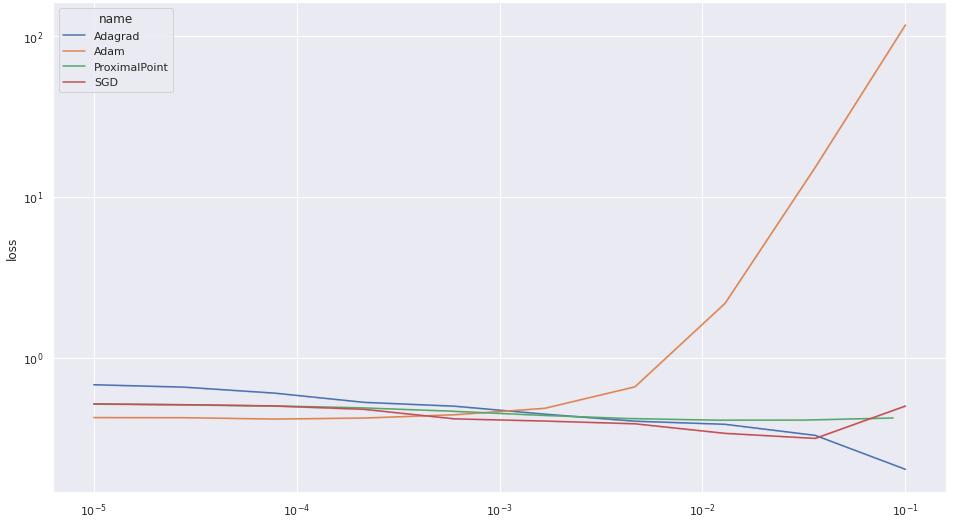
It’s quite apparent that the performance of the proximal point algorithm is quite consistent over the various step-size choices. We also see that Adam’s performance degrades when the step-size is too large. Consequently, to see the difference between the various algorithms more clearly, let’s plot the results without Adam:
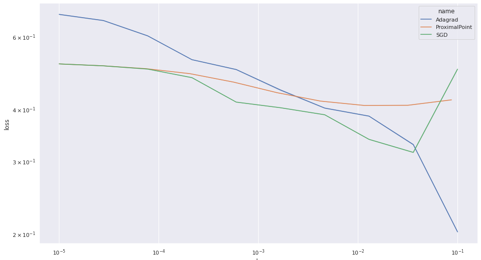
Well, as we see, the proximal point’s performance is the most consistent accross various step-sizes, but it is certainly not the best algorithm for training a factorization machine on this dataset. It appears that Adagrad is.
One possible explanation is that the proximal point algorithm converges more slowly, and requires more epochs to achieve good performance. Let’s test this hypothesis, and run the proximal point algorithm for 50 epochs. And after a few days, I got:
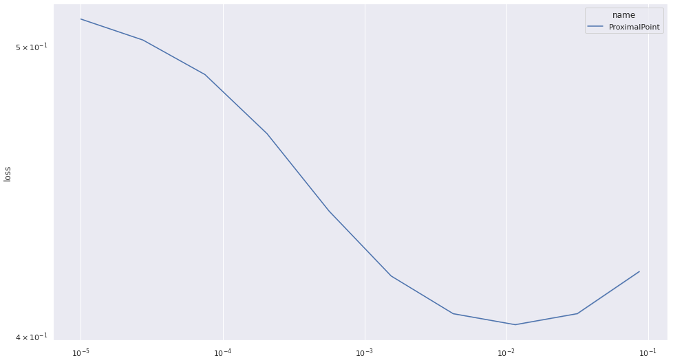
The situation doesn’t seem to improve much. The method is quite consistent in its performance, but it doesn’t seem to converge rapidly to an optimum.
Summary
We have developed an efficiently implementable proximal point step for a highly non-trivial and non-convex problem, and provided an implementation. To the best of my knowledge, this post sets foot in an uncharted territory, and thus I an not sure what is the method converging to, but from these numerical experiments it doesn’t seem to minimize the average loss. It is my hope that the research community can provide such answers.
Writing this entire series about efficient implementation of incremental proximal point methods has been extremely fun and I certainly learned a lot about Python, PyTorch, and better understood the essence of these methods. I hope that you, the readers, enjoyed as much as I did. It’s time for new adventures! I don’t know what the next post will be about, but I’m sure it will be fun!
-
Steffen Rendle (2010), Factorization Machines, IEEE International Conference on Data Mining (pp. 995-1000) ↩
-
It follows from the fact that \(h(t)=\ln(1+\exp(t))\) and \(h^*(s)=s\ln(s)+(1-s)\ln(1-s)\) are both Legendre-type functions: essencially smooth and strictly-convex function. ↩
-
seperability is the fact that \(\displaystyle \min_{x_1,x_2} f(x_1) + g(x_2) = \min_{x_1} f(x_1) + \min_{x_2} g(x_2)\). ↩