“Proximal Point - warmup"
This post is part of the series "Proximal point", and is not self-contained.
Series posts:
- “Proximal Point - warmup" (this post)
-
“Proximal point - convex on linear losses"
-
“Proximal Point - regularized convex on linear I"
-
“Proximal Point - regularized convex on linear II"
-
“Proximal Point is, after all, yet another gradient method"
-
“Selective approximation - the prox-linear method for training arbitrary models"
-
“Proximal Point with Mini Batches"
-
“Proximal Point with Mini Batches - Convex On Linear"
-
“Proximal Point with Mini Batches - Regularized Convex On Linear"
-
“Proximal Point to the Extreme - Factorization Machines"
- “Proximal Point - warmup" (this post)
- “Proximal point - convex on linear losses"
- “Proximal Point - regularized convex on linear I"
- “Proximal Point - regularized convex on linear II"
- “Proximal Point is, after all, yet another gradient method"
- “Selective approximation - the prox-linear method for training arbitrary models"
- “Proximal Point with Mini Batches"
- “Proximal Point with Mini Batches - Convex On Linear"
- “Proximal Point with Mini Batches - Regularized Convex On Linear"
- “Proximal Point to the Extreme - Factorization Machines"
Intro
I have two desires - learning Python, and sharing my thoughts and learnings on the intersection between software, mathematical optimization, and machine learning in an accessible manner to a wide audience. So let’s begin our mutual adventure with a few simple ideas, which are heavily inspired by a great work by Asi and Duchi1.
When training machine-learning models, we typically aim to minimize the training loss
\[\frac{1}{n} \sum_{k=1}^n f_k(x),\]where \(f_k\) is the loss of the \(k^{\mathrm{th}}\) training sample with respect to the model parameter vector \(x\). We usually do that by variants of the stochastic gradient method: at iteration \(t\) we select \(f \in \{ f_1, \dots, f_n \}\), and perform the gradient step \(x_{t+1} = x_t - \eta \nabla f(x_t)\). Many variants exist, i.e. AdaGrad and Adam, but they all share one property - they use \(f\) as a ‘black box’, and assume nothing about \(f\), except for being able to compute its gradient. In this series of posts we explore methods which can exploit more information about the losses \(f\).
For some machine learning practitioners the notation may seem unusual - \(x\) denotes the model’s parameters, rather than the input data. Since this blog focuses on optimization and refers to many papers in the field, I adopted the ubituitous notation in the optimization community, and in mathematics in general - the ‘unknown’ we are looking for is denoted by \(x\). In our context, the ‘unknown’ is the model’s parameter vector. Get used to it :)
Gradient step revisited
The gradient step is usually taught as ‘take a small step in the direction of the negative gradient’, but there is a different view - the well-known2 proximal view:
\[x_{t+1} = \operatorname*{argmin}_{x} \left\{ H_t(x) \equiv \color{blue}{f(x_t) + \nabla f(x_t)^T (x - x_t)} + \frac{1}{2\eta} \color{red}{\| x - x_t\|_2^2} \tag{*} \right\}.\]The blue part in the formula above is the tangent, or the first-order Taylor approximation at \(x_t\), while the red part is a measure of proximity to \(x_t\). In other words, the gradient step can be interpreted as
find a point which balances between descending along the tangent at \(x_t\), and staying in close proximity to \(x_t\).
The balance is controlled by the step-size parameter \(\eta\). Larger \(\eta\) puts less emphasis on the proximity term, and thus allows us to take a step farther away from \(x_t\).
To convince ourselves that \((\text{*})\) above is indeed the gradient step in disguise, we recall that by Fermat’s principle we have \(\nabla H_t(x_{t+1}) = 0\), or equivalently
\[\nabla f(x_t) + \frac{1}{\eta} (x_{t+1} - x_t) = 0.\]By re-arranging and extracting \(x_{t+1}\) we recover the gradient step.
Beyond the black box
A first order approximation is reasonable if we know nothing about the function \(f\), except for the fact that it is differentiable. But what if we do know something about \(f\)? Let us consider an extreme case - we would like to exploit as much as we can about \(f\), and define
\[x_{t+1} = \operatorname*{argmin}_x \left\{ \color{blue}{f(x)} + \frac{1}{2\eta} \color{red}{\|x - x_t\|_2^2} \right\}\]The idea is known as the stochastic proximal point method3, or implicit learning4. Note, that when the loss \(f\) is “too complicated”, we might not have any efficient method to compute \(x_{t+1}\), which makes this method impractical for many types of loss functions, i.e. training deep neural networks. However, it turns out to be useful for many losses. In the following series of posts we will explore ways to efficiently implement the method for some losses families, and demonstrate the method’s advantages over regular black-box approaches. We will begin our implementation endaevor from a simple example, the linear least-squares problem, and eventually reach more advanced scenarios, such as training factorization machines and neural networks.
Now, let’s talk about implementing the method for linear regression. Our aim is to minimize
\[\frac{1}{2n} \sum_{k=1}^n (a_i^T x + b_i)^2 \tag{LS}\]Thus, every \(f\) is of the form \(f(x)=\frac{1}{2}(a^T x + b)^2\), and our computational steps are of the form:
\[x_{t+1}=\operatorname*{argmin}_x \left\{ P_t(x)\equiv \frac{1}{2}(a^T x + b)^2 + \frac{1}{2\eta} \|x - x_t\|^2 \right\} \tag{**}\]Now it becomes a bit technical, so bear with me - it leads to an important conclusion at the end of this post. To derive an explicit formula for \(x_{t+1}\) let’s solve the equation \(\nabla P_t(x_{t+1}) = 0\):
\[a(a^T x_{t+1} + b) + \frac{1}{\eta}(x_{t+1} - x_t) = 0\]Re-arranging, we obtain
\[[\eta (a a^T) + I] x_{t+1} = x_t - (\eta b) a\]Solving for \(x_{t+1}\) leads to
\[x_{t+1} =[\eta (a a^T) + I]^{-1}[x_t - (\eta b) a].\]It seems that we have defeated the whole point of using a first-order method - simple and efficient formula for computing \(x_{t+1}\) from \(x_t\). Here we seem to have to invert a matrix at every step of the algorithm, which is very inefficient. The remedy comes from the famous Sherman-Morrison matrix inversion formula, which leads us to
\[x_{t+1}=\left[I - \frac{\eta a a^T}{1+\eta \|a\|_2^2} \right][x_t - (\eta b) a],\]which by tedious, but simple mathematical manipulations can be further simplified into
\[x_{t+1}=x_t - \underbrace{\frac{\eta (a^T x_t+b)}{1+\eta \|a\|_2^2}}_{\alpha_t} a. \tag{S}\]Ah! Finally! Now we have arrived at a formula which can be implemented in \(O(d)\) operations, where \(d\) is the dimension of \(x\). We just need to compute the coefficient \(\alpha_t\), and take a step in the direction opposite to \(a\).
An interesting thing to observe here is that large step-sizes \(\eta\) do not lead to an overly large coefficient \(\alpha_t\), since \(\eta\) appears both in the numerator and the denominator. Intuitively, this might lead to a more stable learning algorithm - it is less sensitive bad step-size choice. In fact, this stability property extends beyond least-squares problems, which is the subject of the excellent paper1 by Asi and Duchi which inspired me to write.
Let’s implement out optimizer in Python, using PyTorch. Despite looking somewhat un-natural, PyTorch was chosen for two reasons: first, I would like to learn PyTorch; second, as we move to more generic optimizers in future posts, using PyTorch will become natural. So here it is:
import torch

class LeastSquaresProxPointOptimizer:
    def __init__(self, x, step_size):
        self._x = x
        self._step_size = step_size

    def step(self, a, b):
        # helper variables
        x = self._x
        step_size = self._step_size

        # compute alpha
        numerator = step_size * (torch.dot(a, x) + b).item()
        denominator = 1 + step_size * torch.dot(a, a).item()
        alpha = numerator / denominator

        # perform step
        x.sub_(alpha * a)
Now, for example, if we want to solve the linear least-squares problem:
\[\min_x \quad \frac{1}{2}(-x_1+x_2-1)^2+\frac{1}{2}(x_1+x_2-2)^2+\frac{1}{2}(x_1-2x_2)^2\]We can use our optimizer in the following manner:
import torch
import random

# each tuple in the list is (a, b)
data = [(torch.tensor([-1., 1.]), -1.),
        (torch.tensor([1., 1.]), -2.),
        (torch.tensor([1., -2.]), 0.)]

# setup the optimizer
x = torch.empty(2)
torch.nn.init.normal_(x)
opt = LeastSquaresProxPointOptimizer(x, step_size=1)

# train our parameter vector `x`
num_of_epochs = 20
for epoch in range(0, num_of_epochs):
    for a, b in random.sample(data, len(data)):
        opt.step(a, b)

# print the parameters
print(x)
So, now we are ready for a more serious experiment.
Experiment
We will compare the performance of our method against several optimizers which are widely used in existing machine learning frameworks: AdaGrad, Adam, SGD, and will test the stability of our algorithm w.r.t the step-size choice, since our intuition suggested that our method might be more stable than the ‘black box’ approaches. The Python code for my experiments can be found in this git repo.
We use the Boston Housing Dataset to test our algorithms on a linear regression model attempting to predict housing prices \(y\) based on the data vector \(p \in \mathbb{R}^3\) comprising the number of rooms, population lower status percentage, and average pupil-teacher ratio by the linear model:
\[y = p^T \beta +\alpha\]To that end, we will attempt to minimize the mean squared error over all our samples \((p_j, y_j)\), namely:
\[\min_{\alpha, \beta} \quad \frac{1}{2n} \sum_{j=1}^n (p_j^T \beta +\alpha-y_j)^2\]In terms of (LS) above , we have the parameters \(x = (\beta_1, \beta_2, \beta_3, \alpha)^T\), and the data \(a_i = (p_{i,1}, p_{i,2}, p_{i,3}, 1)^T\), and \(b_i = -y_i\).
Let’s look at the results! Below is a chart obtained by running each method for 100 epochs, taking the best training loss, and repeating each experiment 20 times for each of our step-size choices. Each line is the average of the best obtained loss of each experiment run. The x-axis is the step-size, while the y-axis is the deviation of the obtained training loss from the optimal loss (recall - least squared problems can be solved efficiently and exactly solved using a direct method).
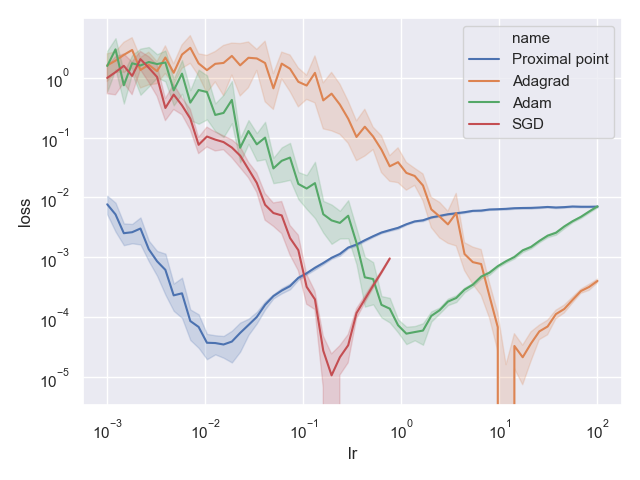
What we observe is interesting - all optimizers except for our proximal point optimizer may produce solutions which are far away from the optimum, but there is a narrow choice of step-sizes for which they produce a solution which is very close to the optimum. In particular, AdaGrad with a step-size of around \(\eta=10\) produces a solution which is practically optimal - its deviation from the optimum is almost 0 (note the log-scale). On the other hand, the proximal point optimizer behaves fairly well for a huge range of step-sizes, from \(10^{-3}\) up to \(10^2\)! Its deviation from the optimal loss remains quite small.
Conclusion
We gave up the black box and made our hands dirty by devising a custom optimizer for least-squares problems which treats the losses directly, without approximating. In return, we gained stability w.r.t the step-sizes. Namely, to obtain a reasonably good model, we do not need to invest a lot of computational effort into scanning a large set of hyperparameter choices.
The need to devise a custom optimizer for each problem in machine learning, which may require some serious mathematical trickery, might make such methods quite prohibitive and poses a serious barrier between machine learnign practicioners and stable learning methods. Furthermore, for many machine learning problems it is not even possible to devise a simple formula for computing \(x_{k+1}\). In the next blog post we will attempt to make a crack in this barrier by devising a more generic approach, and implementing a PyTorch optimizer based on our mathematical developments. Stay tuned!
References
-
Asi, H. & Duchi J. (2019). Stochastic (Approximate) Proximal Point Methods: Convergence, Optimality, and Adaptivity SIAM Journal on Optimization 29(3) (pp. 2257–2290) ↩ ↩2
-
Polyak B. (1987). Introduction to Optimization. Optimization Software ↩
-
Bianchi, P. (2016). Ergodic convergence of a stochastic proximal point algorithm. SIAM Journal on Optimization, 26(4), 2235-2260. ↩
-
Kulis, B., & Bartlett, P. L. (2010). Implicit online learning. In Proceedings of the 27th International Conference on Machine Learning (ICML-10) (pp. 575-582). ↩