“Proximal Point with Mini Batches - Convex On Linear"
This post is part of the series "Proximal point", and is not self-contained.
Series posts:
-
“Proximal Point - warmup"
-
“Proximal point - convex on linear losses"
-
“Proximal Point - regularized convex on linear I"
-
“Proximal Point - regularized convex on linear II"
-
“Proximal Point is, after all, yet another gradient method"
-
“Selective approximation - the prox-linear method for training arbitrary models"
-
“Proximal Point with Mini Batches"
- “Proximal Point with Mini Batches - Convex On Linear" (this post)
-
“Proximal Point with Mini Batches - Regularized Convex On Linear"
-
“Proximal Point to the Extreme - Factorization Machines"
- “Proximal Point - warmup"
- “Proximal point - convex on linear losses"
- “Proximal Point - regularized convex on linear I"
- “Proximal Point - regularized convex on linear II"
- “Proximal Point is, after all, yet another gradient method"
- “Selective approximation - the prox-linear method for training arbitrary models"
- “Proximal Point with Mini Batches"
- “Proximal Point with Mini Batches - Convex On Linear" (this post)
- “Proximal Point with Mini Batches - Regularized Convex On Linear"
- “Proximal Point to the Extreme - Factorization Machines"
Last time we introduced the mini-batch version of the stochastic proximal point method, and its specialization to the convex-on-linear setup with the mini-batch \(B\):
\[x_{t+1} = \operatorname*{argmin}_x \left \{ \frac{1}{|B|} \sum_{i \in B} \phi(a_i^T x + b_i) + \frac{1}{2\eta} \|x - x_t\|_2^2 \right\}.\]Then, using a more general version of convex duality we saw that the above is equivalent to maximizing the dual function
\[q(s) = -\frac{\eta}{2} \|A_B^T s\|_2^2 + (A_B x_t + b_B)^T s - \frac{1}{|B|} \sum_{i \in B} \phi^*(|B| s_i),\]where \(A_B\) and \(b_B\) are obtained by vertical concatenation of \(a_i^T\) and \(b_i\) for \(i \in B\).
Focusing on the essentials
Before digging deeper, to simplify notation we first transform the maximization problem to an equivalent minimization problem. To that end, we do the following transformation:
\[q(s) = - \left( \frac{1}{2} \left \| \sqrt{\eta} A_B^T s \right \|_2^2 - (A_B x_t + b_B)^T s + \frac{1}{\vert B \vert} \sum_{i \in B} \phi^*(\vert B\vert s_i) \right)\]Recalling that maximizing a function is equivalent to minimizing its negation, and denoting \(P=\sqrt{\eta} A_B^T\), \(c = -(A_b x_t + b_B)\), and \(m = \vert B \vert\), we obtain that we aim to minimize functions of the form
\[\tilde{q}(s)=\frac{1}{2} \|P s\|_2^2 + c^T s + \frac{1}{m} \sum_{i \in B} \phi^*(m s_i). \tag{DM}\]Recall, also, that the algorithm for computing \(x_{t+1}\) comprises the following steps:
- Compute the parameters of the dual problem: \(P\), and \(c\).
- Find a maximizer \(s^*\) of \(q(s)\), which is also a minimizer of \(\tilde{q}(s)\) above.
- Compute \(x_t - \eta A_B^T s^*\).
The first and last steps can be computed by a generic optimizer, while the second step depends on \(\phi\) and has to be computed by specialized code. So, here is our generic optimizer
import torch

class MiniBatchConvLinOptimizer:
    def __init__(self, x, step_size, phi):
        self._x = x
        self._step_size = step_size
        self._phi = phi

    def step(self, A_batch, b_batch):
        # helper variables
        x = self._x
        step_size = self._step_size
        phi = self._phi

        # compute dual problem coefficients
        P = math.sqrt(step_size) * A_batch.t()
        c_neg = torch.addmv(b_batch, A_batch, x)

        # solve dual problem
        s_star = phi.solve_dual(P, c_neg)

        # perform step
        step_dir = torch.mm(A_batch.t(), s_star)
        x.sub_(step_size * step_dir.reshape(x.shape))

        # return the losses w.r.t the params before making the step
        return phi.eval(c_neg)
We can also immediately implement the corresponding phi for \(L2\) losses, namely, for least-squares problems. In that case, the dual problem amounts to solving
or, equivalently, computing
\[s^* = -(P^T P + m I)^{-1} c\]Here is the code:
class L2Loss:
    def solve_dual(self, P, c_neg):
        m = P.shape[1]  # number of columns = batch size
        lsh_mat = torch.addmm(I, P.t(), P, beta=m)

        # solve positive-definite linear system using Cholesky factorization
        lhs_factor = torch.cholesky(lhs_mat)
        rhs_col = c.unsqueeze(1) # make rhs a column vector, so that cholesky_solve works
        return torch.cholesky_solve(rhs_col, lhs_factor)

    def eval(self, lin):
        return 0.5 * (lin ** 2)
Now we can construct a least-squares mini-batch optimizer using:
opt = MiniBatchConvLinOptimizer(x, step_size, L2Loss())
Beyond least squares, i.e. logistic regression, the minimum of \(\tilde{q}\) cannot be computed analytically by a simple closed-form formula. But we are at luck! Minimizing low-dimensional convex functions has been the subject of a few decades of research, and many efficient methods have emerged.
Welcome CVXPY
CVXPY is a Python package for convex optimization, which acts like a kind of a compiler. We specify the optimization problem we want to solve, and the package “compiles” it to a low-level representation which can be passed to a lower-level solver, usually written in C, which solves it. This low level solver is usually referred to as a backend. Examples of such solvers include the open-source solvers SCS and ECOS, the commercial solver MOSEK, and many more.
Entire courses can be, and are taught about convex optimization, and I do not intend to teach another one in this blog. Rather, I intend to introduce unfamiliar readers to the mere existance of this technology, and readers who are interested will be able to learn the subject through one of the available courses, from a book1, or from any other source.
To install CVXPY we can use:
pip install cvxpy
Now we can import and use it. An optimization problem consists of two components - the function we wish to minimize or maximize, called the objective, and the set of constraints subject to which the optimization is done. Let’s solve a simple optimization problem with constraints:
import cvxpy as cp

# define the problem
x = cp.Variable(2) # a two-dimensional variable
objective = cp.sum_squares(cp.vstack([x[0] - x[1] + 1,
                                      x[0] + x[1] - 1,
                                      x[0] - 2*x[1] + 3]))
constraints = [x >= 0, cp.sum(x) == 1]
problem = cp.Problem(cp.Minimize(objective), constraints)

# solve the problem, print the optimal value, and the optimal solution
result = problem.solve()
print(f'Optimal value = {result}, optimal x = {x.value}')
The code is, hopefully, self explanatory, and readers can see that it indeed aims to solve the following optimization problem:
\[\begin{aligned} \min_{x \in \mathbb{R}^2} &\quad (x_1-x_2+1)^2+(x_1+x_2-1)^2+(x_1-2x_2+3)^2 \\ \text{subject to} &\quad x_1,x_2 \geq 0 \\ &\quad x_1+x_2=1 \end{aligned}\]Here is the output of the code above:
Optimal value = 0.9999999999999997, optimal x = [-3.60317695e-19 1.00000000e+00]
This means that the minimum value is \(\approx 1\), and the vector \(x^*\approx(0, 1)\) attains it, meaning it is an optimal solution.
Let’s try to implement the logistic loss using CVXPY. We have \(\phi(z)=\ln(1+\exp(z))\), meaning that \(\phi^*(s) = s \ln(s) + (1-s) \ln(1-s)\). Fortunately, the convex function \(x \ln(x)\) is used in a many optimization problems, and in many cases is recognized by convex optimization packages. It is referred to as the negative entropy function. So here is the code for the logistic loss implementation, which minimizes \(\tilde{q}(s)\) using CVXPY:
import torch
import cvxpy as cp

class LogisticLoss:
    def solve_dual(self, P, c_neg):
        # extract information and convert tensors to numpy. CVXPY
        # works with numpy arrays
        m = P.shape[1]
        P = P.data.numpy()
        c_neg = c_neg.data.numpy()

        # define the dual optimization problem
        s = cp.Variable(m)
        objective = 0.5 * cp.sum_squares(P @ s) - # `@` is a matrix product
                    cp.sum(c_neg * s) -
                    (cp.sum(cp.entr(m * s)) + cp.sum(cp.entr(1 - m * s))) / m
        prob = cp.Problem(cp.Minimize(objective))

    	# solve the problem, and extract the optimal solution
        prob.solve()
        s_star = torch.tensor(s.value).unsqueeze(1)

        return s_star

    def eval(self, lin):
        return torch.log1p(torch.exp(lin))
Now, we can also employ the mini-batch version of the stochastic proximal point method to solve logistic regression problems using the following optimizer:
opt = MiniBatchConvLinOptimizer(x, step_size, LogisticLoss())
Simple logistic regression experiment
First, let’s see that our optimizer produces reasonable results. We will use the same spambase data-set we used before. It is composed of 57 numerical columns, signifying frequencies of various frequently-occuring words, and average run-lengths of capital letters, and a 58-th column with a spam indicator.
Let’s load the data-set, scale its features, and construct a PyTorch data-set object:
import pandas as pd
from sklearn import preprocessing
from torch.utils.data.dataset import TensorDataset

url = 'https://web.stanford.edu/~hastie/ElemStatLearn/datasets/spam.data'
df = pd.read_csv(url, delimiter=' ', header=None)

min_max_scaler = preprocessing.MinMaxScaler()
scaled = min_max_scaler.fit_transform(df.iloc[:, 0:56])
df.iloc[:, 0:56] = scaled

W = torch.tensor(np.array(df.iloc[:, 0:56])) # features
Y = torch.tensor(np.array(df.iloc[:, 57]))   # labels
ds = TensorDataset(W, Y)
Now, let’s train a logistic regression model for classifying spam based on the features in the data-set, with batches of 4 samples.
# init. model parameter vector
x = torch.empty(56, requires_grad=False, dtype=torch.float64)
torch.nn.init.normal_(x)

# create optimizer
step_size = 1
opt = MiniBatchConvLinOptimizer(x, step_size, LogisticLoss())

# run 40 epochs, print out data loss and reg. loss
for epoch in range(40):
  loss = 0.0
  for w, y in DataLoader(ds, shuffle=True, batch_size=4):
	A_batch = (1 - 2*y) * w
    b_batch = torch.zeros_like(a)
    losses = opt.step(A_batch, b_batch)

    loss += torch.sum(losses).item()

  print(f'epoch = {epoch}, loss = {loss / len(ds)}')
I obtained the following output:
epoch = 0, loss = 0.49779446008581707
epoch = 1, loss = 0.37720419193721605
...
epoch = 37, loss = 0.24126466392084467
epoch = 38, loss = 0.24089484987149695
epoch = 39, loss = 0.24035799118074533
Making it faster
If you ran the code above, you may have noticed that it is quite slow.We can make it a bit faster by utilizing more powerful features of CVXPY. Recall, that CVXPY is just a ‘compiler’ which transforms the problem we provide into a lower-level form. The optimization problems of minimizing \(\tilde{q}(s)\) share similar structure - they only differ in the matrix \(P\) and the vector \(c\). But every call to the solve_dual method constructs a new optimization problem, which is compiled every time we invoke that method.
CVXPY lets us compile a family of problems sharing the same structure once, and re-use it every time we need to solve it with different data. Objects of cvxpy.Parameter are used as placeholders for the problem data, and can be used instead of the actual data. The problem can then be constructed once, and re-used by assigning values to the parameters.
Another improvement comes from elementary linear algebra:
\[\frac{1}{2} \|P s\|_2^2=\frac{1}{2} s^T (P^T P) s.\]The size of the matrix \(P\) is \(d \times m\), where \(d\) is the dimension of the training data and \(m\) is the mini-batch size. The above means that we can formulate our optimization problems in terms of the quadratic matrix \(P^T P\) of size is \(m\times m\), which does not depend on the dimension of the training data. Consequently we can compute this matrix as a PyTorch tensor, and use it to construct the CVXPY problem, which now also becomes independent on the dimension of the training data.
Here is an implementation of the logistic loss based on the combination of both idea:
class LogisticLoss:
    def __init__(self, batch_size):
        self.PTP = cp.Parameter((batch_size, batch_size), PSD=True)
        self.c_neg = cp.Parameter(batch_size)
        self.batch_size = batch_size
        self.prob, self.s = LogisticLoss._build_problem(self.PTP, self.c_neg, batch_size)

    @staticmethod
    def _build_problem(PTP, c_neg, m):
        s = cp.Variable(m)
        objective = 0.5 * cp.quad_form(s, PTP) - cp.sum(c_neg * s) - (cp.sum(cp.entr(m * s)) + cp.sum(cp.entr(1 - m * s))) / m
        prob = cp.Problem(cp.Minimize(objective))

        return prob, s

    def solve_dual(self, P, c_neg):
        PTP = torch.mm(P.t(), P)
        m = PTP.shape[0]

        if m == self.batch_size:
            prob, s = self._reuse(PTP, c_neg)
        else:
            prob, s = self._build_new(PTP, c_neg, m)

        return self._solve(prob, s)

    @staticmethod
    def _solve(prob, s):
        # ECOS/SCS/MOSEK are capable of dealing with the dual problem at hand
        # MOSEK is a commercial-grade solver and is the most reliable,
        # and is free for academic use!
        prob.solve(cp.MOSEK)
        s_star = torch.from_numpy(s.value).unsqueeze(1)
        return s_star

    @staticmethod
    def _build_new(PTP, c_neg, m):
        prob, s = LogisticLoss._build_problem(PTP.data.numpy(), c_neg.data.numpy(), m)
        return prob, s

    def _reuse(self, PTP, c_neg):
        self.PTP.value = PTP.data.numpy()
        self.c_neg.value = c_neg.data.numpy()
        prob = self.prob
        s = self.s
        return prob, s

    def eval(self, lin):
        return torch.log1p(torch.exp(lin))
On my computer, it is approximately 1.5 times faster. Not too impressive, but any gain is a gain. We could make it faster by exploiting the lower-level facilities provided by CVXPY. But the only plausible way of making it really fast is building a custom optimization solver for the logistic losses’ dual problem, which fully exploits the structure of the problem. This is what we would have done if we were to implement a production-grade optimizer.
Building such a solver is beyond the scope of this blog post, but there are several resources1 interested readers might consider. A specialized solver could solve the dual problem, even for batches of size 256, in a few milliseconds.
Note, that computing \(P^T P\) costs \(\mathcal{O}(d m^2)\) operations. Assuming that model dimensions are large, while the mini-batch size is small, this part dominates the computational complexity of computing \(x_{t+1}\). To be fair, we should point out that regular SGD with mini-batches costs only \(\mathcal{O}(d m)\) time, so we should use the proximal point algorithm when its benefits, such as cheaper hyperparameter tuning, outweigh the above-mentioned cost.
Stability experiment
Let’s see if for our logistic regression problem we are getting a stable algorithm. As previously, for each step size and for each batch size we run several experiments. Then, we show the results in a loss vs. step size plot.
I chose to use Python’s multiprocessing capabilities to make the experiment faster, and be able to utilize a cloud service with many CPUs to parallelize work. So here is the code which runs the experiment and plots the results. We use a multiprocessing pool to run an asynchronous task for every combination of the experiment parameters, and use a queue to feed the results of each epoch from the parallel executions back to the main program.
import seaborn as sns
import matplotlib.pyplot as plt
import torch.multiprocessing as mp

# define experiment setup
batch_sizes = [1, 2, 3, 4, 5, 6]
experiments = range(10)
epochs = range(10)
step_sizes = np.geomspace(0.001, 100, 10)

# construct multiprocessing data exchange objecgts
manager = mp.Manager()
queue = manager.Queue()

# run experiments
print('Starting parallel training experiments')
pool = mp.Pool(processes=6)
params = [
    (queue, dataset, epochs, step_size, batch_size, experiment)
    for step_size in step_sizes
    for batch_size in batch_sizes
    for experiment in experiments
]
res = pool.starmap_async(train, params, chunksize=1)

# wait for results to arrive
print('Gathering results from parallel experiments')
losses = []
total_epochs = len(batch_sizes) * len(experiments) * len(step_sizes) * len(epochs)
for i in tqdm(range(total_epochs), desc='Training', unit='epochs', ncols=160, smoothing=0.05):
    losses.append(queue.get())

print('Waiting for parallel jobs to end')
res.wait(timeout=1)
losses = pd.concat(losses)

losses.to_csv('losses.csv')

best_losses = losses[['batch_size', 'step_size', 'experiment', 'loss']]\
    .groupby(['batch_size', 'step_size', 'experiment'], as_index=False)\
    .min()

sns.set()
ax = sns.lineplot(x='step_size', y='loss', hue='batch_size', data=best_losses, err_style='band', legend='full')
ax.set_yscale('log')
ax.set_xscale('log')
plt.show()
And here is the train function called on line 24, which actually trains a model with the given parameters, and feeds the results of each epoch through the queue back to the main program.
def train(queue, dataset, epochs, step_size, batch_size, experiment):
    x = torch.empty(56, requires_grad=False, dtype=torch.float64)
    torch.nn.init.normal_(x)

    optimizer = MiniBatchConvLinOptimizer(x, step_size, LogisticLoss(batch_size=batch_size))
    successful = True
    for epoch in epochs:
        epoch_loss = 0.
        for w, y in torch.utils.data.DataLoader(dataset, shuffle=True, batch_size=batch_size):
            # logistic regression input in "convex-on-linear" form
            sign = (1 - 2 * y.unsqueeze(1))
            A_batch = sign * w
            b_batch = torch.zeros_like(y, dtype=x.dtype)

            batch_losses = optimizer.step(A_batch, b_batch)
            epoch_loss += torch.sum(batch_losses).item()

        epoch_loss /= len(dataset)
        df = pd.DataFrame.from_dict(
                {'batch_size': [batch_size],
                 'step_size': [step_size],
                 'experiment': [experiment],
                 'epoch': [epoch],
                 'loss': [epoch_loss]})
        queue.put(df)
After a few hours, I obtained the following result:
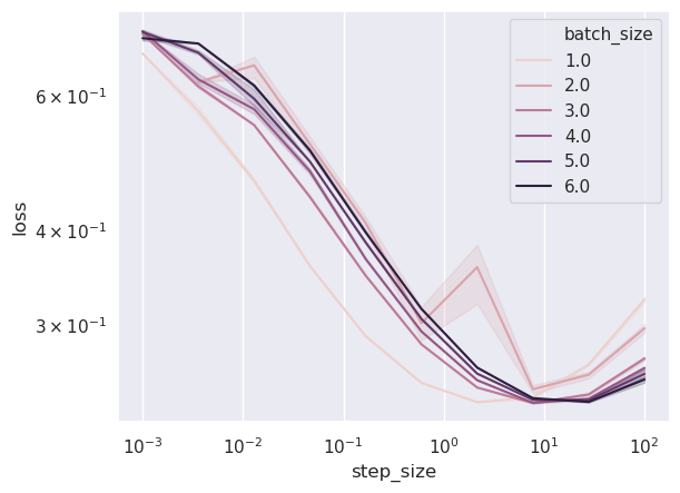
When the step sizes are too small, in this case less than \(10\), convergence is slow and we are not able to converge to a solution achieving a training loss below \(3\times 10^{-1}\) - our 10 epochs are not enough. When the step size becomes larger, the benefit of mini-batching becomes apparent - larger batch size, which appears as a darker color, leads to a better training loss. The stability property remains - we do not diverge, and we obtain a solution with a reasonable training loss for a huge range of step sizes: from as small as 0.1 to as large as 100!
Teaser
We have gone through a very long journey, and explored a variety of cases for which the proximal point approach of using the losses instead of approximating leads to a practically implementable algorithm. When training on a single sample at a time, our most general algorithm was aimed at convex-on-linear losses with regularization. Note, that in this post we did not deal with regularized losses, and that is exactly the subject of the next post - mini-batch training for convex-on-linear losses with regularization.
As a final remark, I would like to thank the MOSEK generous help with debugging some of the issues I had when I wrote the code for this blog post.