“Proximal Point - regularized convex on linear I"

We continue our endeavor of looking for a practical and efficient implementation of the stochastic proximal point method, which aims to minimize the average loss \(\frac{1}{n} \sum_{i=1}^n f_i(x)\) over \(n\) training samples by, iteratively, selecting \(f \in \{f_1, \dots, f_n \}\) and computing

\[x_{t+1} = \operatorname*{argmin}_x \left\{ f(x) + \frac{1}{2\eta} \|x - x_t\|_2^2 \right \}.\]

Recall, the challenge lies in the fact that \(f\) can be arbitrary complex, and thus computing \(x_{t+1}\) can be arbitrarily hard, and may even be impossible. A major benefit, on the othet hand, is stability w.r.t step-size choices, compared with black-box stochastic gradient methods.

In the previous post we derived, implemented, and tested an efficient implementation for a specific family of losses of the form

\[f(x)=\phi(a^T x + b),\]

where \(\phi\) is a convex function. Such losses include, for example, linear least squares and logistic regression. In this post we add a convex regularizer \(r(x)\), and discuss losses of the following form:

\[f(x)=\phi(a^T x + b) + r(x).\]

For example, consider an L2 regularized least-squares problem:

\[\min_x \quad \frac{1}{2 n} \sum_{i=1}^n (a_i^T x + b_i)^2 + \frac{\lambda}{2} \|x\|_2^2.\]

The above problem is an instance of regularized convex-on-linear losses with \(\phi(t)=\frac{1}{2} t^2\) and \(r(x) = \frac{\lambda}{2} \|x\|_2^2\), both are known to be convex functions.

L2 regularization

Suppose that \(r(x)=(\lambda/2) \|x\|_2^2\), namely, we may consider an L2 regularized least squares or an L2 regularized logistic regression problem. Let’s repeat the steps we have done in the previous post, and see if we obtain similar results - decoupling a ‘generic’ optimizer from some minimal user-provided knowledge about \(\phi\).

We would like to compute \(x_{t+1}\) by solving the following problem using convex duality theory:

\[x_{t+1} = \operatorname*{argmin}_{x} \left\{ \phi(a^T x + b) + \frac{\lambda}{2} \|x\|_2^2+\frac{1}{2\eta} \|x - x_t\|_2^2 \right\}.\]

Defining the auxiliary variable \(u = a^T x + b\), we obtain the problem of minimizing the following over \(x\) and \(u\):

\[\phi(u)+ \frac{\lambda}{2} \|x\|_2^2+\frac{1}{2\eta} \|x - x_t\|_2^2 \qquad \text{subject to} \qquad u = a^T x + b.\]

The corresponding dual problem aims to maximize

\[\begin{align} q(s) &= \inf_{x,u} \left \{ \phi(u)+ \frac{\lambda}{2} \|x\|_2^2+\frac{1}{2\eta} \|x - x_t\|_2^2 + s(a^T x + b - u) \right \} \\ &= \color{blue}{ \inf_x \left \{ \frac{\lambda}{2} \|x\|_2^2+\frac{1}{2\eta} \|x - x_t\|_2^2 + s a^T x \right \}} + \color{red}{\inf_u \left\{ \phi(u) - s u \right\}} + s b \end{align}\]

Recalling the previous post, the red part is \(-\phi^*(s)\), where \(\phi^*\) is the convex conjugate function of \(\phi\). The blue part is a simple quadratic minimization problem, which can be solved by equating the gradient of the term inside the \(\inf\) with zero. We save the tedious (and quite lengthy!) math, and state only the final results. The minimizer is

\[x = \frac{1}{1 + \lambda \eta} (x_t - \eta s a),\]

and the minimum is

\[-\frac{\eta \|a\|_2^2}{2(1+\lambda \eta)} s^2 + \frac{a^T x_t}{1 + \lambda \eta} s + CONST\]

where \(CONST\) are terms which do not depend on \(s\) and thus we don’t care what they are. Consequently, dual problem aims to maximize the following one-dimensional function (up to a constant):

\[q(s)=-\frac{\eta \|a\|_2^2}{2(1+\lambda \eta)} s^2 + \left[\frac{a^T x_t}{1 + \lambda \eta} + b \right] s - \phi^*(s).\]

Viola! We arrived at the expected result, and reduced the problem of computing \(x_{t+1}\) to a simple one-dimensional problem which depends only on \(\phi\). The corresponding “generic” algorithm for computing \(x_{t+1}\) is:

1. Compute the coefficients of \(q(s)\), namely, \(\alpha = \frac{\eta \|a\|_2^2}{1+\lambda \eta}\) and \(\beta = \left[\frac{a^T x_t}{1 + \lambda \eta} + b \right]\).
2. Find a maximizer \(s^*\) of \(q(s)=-\frac{\alpha}{2} s^2 + \beta s - \phi^*(s)\).
3. Compute \(x_{t+1} = \frac{1}{1 + \lambda \eta} (x_t - \eta s^* a)\)

But is our algorithm really generic? The reality is that it is not. The regularizer is deeply integrated in all computational steps - given a different regularizer, steps (1) and (3) can be radically different from the above.

Unfortunately, it is not possible to easily decouple the regularizer away, but it is possible to provide a formula for \(q(s)\) composed of concepts which a practitioner can find in a textbook, and thus does not have to re-derive a dual problem for every regularizer. Deriving such a formula will be the subject of our next post. To avoid making a lengthy post, we devote the rest of this post to implementing and experimenting with an optimizer tailored for L2 regularisation.

Code and experiment

Let’s implement the optimizer we just derived. The functions \(\phi\) are represented in the same way as in the previous post - a function which solves the dual problem of maximizing \(q(s)\). The optimizer’s job is to construct the coefficients \(\alpha, \beta\), run the dual problem solver to obtain \(s^*\), and compute \(x_{t+1}\). For completeness, we include the code, which differs from the optimizer in the previous post by the lines marked by the comment.

import torch

class ConvexOnLinearL2RegSPP:
    def __init__(self, x, eta, regcoef, phi):
        self._eta = eta
        self._phi = phi
        self._regcoef = regcoef
        self._x = x
        
    def step(self, a, b):
        """
        Performs the optimizer's step, and returns the loss incurred.
        """
        eta = self._eta
        regcoef = self._regcoef
        phi = self._phi  
        x = self._x
        
        # compute the dual problem's coefficients
        alpha = eta * torch.sum(a**2) / (1 + eta * regcoef) 
        beta = torch.dot(a, x) / (1 + eta * regcoef) + b
        
        # compute the loss function value
        val = phi.eval(torch.dot(a, x).item()) + (reg_coef / 2) * (x.pow(2).sum().item()) 
        
        # solve the dual problem
        s_star = phi.solve_dual(alpha.item(), beta.item())
        
        # update x
        x.sub_(eta * s_star * a)
        
        return val
    
    def x(self):
        return self._x
        

The various functions \(\phi\) are implemented in the same manner as in the previous post. For completeness, we include the functions from the previous post for the squared loss \(\phi(t) = \frac{1}{2} t^2\) and the logistic loss \(\phi(t)=\log(1+\exp(t))\).

import torch
import math

# 0.5 * t^2
class SquaredSPPLoss:
    def solve_dual(self, alpha, beta):
        return beta / (1 + alpha)
    
    def eval(self, beta):
        return 0.5 * (beta ** 2)
    
    
# log(1+exp(t))
class LogisticSPPLoss:
    def solve_dual(self, alpha, beta):
        def qprime(s):
            -alpha * s + beta + math.log(1-s) - math.log(s)
        
        # compute [l,u] containing a point with zero qprime
        l = 0.5
        while qprime(l) <= 0:
            l /= 2
        
        u = 0.5
        while qprime(1 - u) >= 0:
            u /= 2
        u = 1 - u
        
        while u - l > 1E-16: # should be accurate enough
            mid = (u + l) / 2
            if qprime(mid) == 0:
                return mid
            if qprime(l) * qprime(mid) > 0:
                l = mid
            else:
                u = mid
        
        return (u + l) / 2
   
    def eval(self, beta):
        return math.log(1+math.exp(beta))

Experiment

We use the same adult income dataset from the previous post, but this time learn L2 regularized logistic regression with regularization coefficient \(\lambda=0.1\). Full code can be found in this git repo. Both the above SPP optimizer and PyTorch’s built-in AdaGrad optimizer are used to train the model for 20 epochs several times, each with a different random shuffle of the data. The best training loss of each attempt and each step-size is plotted:

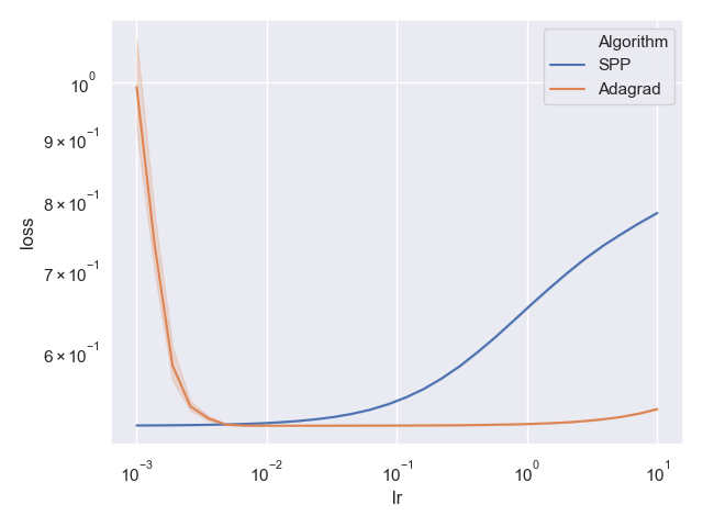
Whoa! Surprise! Our stable stochastic proximal point optimizer has been outperformed by AdaGrad! Both seem to be quite stable, but AdaGrad performs well for a much wider step-size choice. Turns out that adding regularization also ‘regularizes’ a generic black-box optimizer. The key is, I believe, the better conditioning of the optimization problem. We may even talk about it in a future post, but for now we will continue with the proximal point approach.

Teaser

What if we want to regularize using L1 regularization, namely, \(r(x)=\lambda \|x\|_1\)? Such regularizers are especially beneficial when we need a simple model with a small number of features, since they promote a sparse vector \(x\). But it turns out AdaGrad, and other black-box optimizers do not shine so well with L1 regularization, but the proximal point approach does. So we continue our endaevor for an efficient implementation of the approach with a general regularizer \(r\).

Repeating the dual problem derivation for a generic regularizer \(r(x)\) we obtain

\[q(s) = \color{blue}{ \inf_x \left \{ r(x)+\frac{1}{2\eta} \|x - x_t\|_2^2 + s a^T x \right \}} -\phi^*(s) + s b\]

The blue part encompasses the dependency on \(r(x)\), and it seems we have to re-derive it for every regularizer. But is it indeed so? It turns out we don’t always have to - it can be expressed in terms of another well-known concept in optimization, similar to the convex conjugate, which we introduce in the next post. That way, a practitioner does not have to perform the tedious and error prone process of deriving the blue part on her own. Instead, she can pick it up from a catalog which can be found in many textbooks or papers. Stay tuned!