“Proximal Point with Mini Batches"
This post is part of the series "Proximal point", and is not self-contained.
Series posts:
-
“Proximal Point - warmup"
-
“Proximal point - convex on linear losses"
-
“Proximal Point - regularized convex on linear I"
-
“Proximal Point - regularized convex on linear II"
-
“Proximal Point is, after all, yet another gradient method"
-
“Selective approximation - the prox-linear method for training arbitrary models"
- “Proximal Point with Mini Batches" (this post)
-
“Proximal Point with Mini Batches - Convex On Linear"
-
“Proximal Point with Mini Batches - Regularized Convex On Linear"
-
“Proximal Point to the Extreme - Factorization Machines"
- “Proximal Point - warmup"
- “Proximal point - convex on linear losses"
- “Proximal Point - regularized convex on linear I"
- “Proximal Point - regularized convex on linear II"
- “Proximal Point is, after all, yet another gradient method"
- “Selective approximation - the prox-linear method for training arbitrary models"
- “Proximal Point with Mini Batches" (this post)
- “Proximal Point with Mini Batches - Convex On Linear"
- “Proximal Point with Mini Batches - Regularized Convex On Linear"
- “Proximal Point to the Extreme - Factorization Machines"
Throughout our journey in the proximal point land we looked for efficient implementations for minimizing the average loss \(\frac{1}{n} \sum_{i=1}^n f_i(x)\) using the stochastic proximal point method: at iteration \(t\), select \(f \in \{f_1, \dots, f_n\}\), and compute
\[x_{t+1} = \operatorname*{argmin}_x \left\{ f(x) + \frac{1}{2\eta} \|x - x_t\|_2^2 \right\}.\]Since for a general function \(f\) the above is intractable, we covered special and interesting functions \(f\) of practical value to the machine learning community: convex on linear, and regularized variants with an L2 and a generic regularizer. For all of the above, we derived an efficient algorithm to compute \(x_{t+1}\), but our derivations shared one thing in common - we only considered training on one sample at each iteration.
Training by exploiting information from one arbitrarily training sample from the entire training set at each iteration is quite noisy. A standard practice is reducing noise by selecting a mini-batch of training samples, and their corresponding incurred losses, at each iteration. In the following sequence of posts we will derive the mini-batch version of the proximal point algorithm, by following along lines similar to our derivation for convex on linear losses.
The proximal view on mini-batching
Let’s begin by re-interpreting the mini-batch version of stochastic gradient descent: at each iteration, select a mini-batch of samples \(B \in \{1, \dots, n\}\) and compute:
\[x_{t+1} = x_t - \frac{\eta}{|B|} \sum_{i \in B} \nabla f_i(x_t),\]Recalling the proximal view we discussed at the beginning of the series, the mini-batch SGD step can be written as
\[x_{t+1} = \operatorname*{argmin}_x \Biggl\{ \color{blue}{\frac{1}{|B|} \sum_{i \in B} f_i(x_t) + \left( \frac{1}{B} \sum_{i \in B} \nabla f_i(x_t) \right)^T(x - x_t)} + \color{red}{\frac{1}{2\eta} \|x - x_t\|_2^2} \Biggr\}.\]The red part is, as usually, a proximal term penalizing the distance from \(x_t\). The blue term is a linear approximation of \(\frac{1}{\vert B \vert} \sum_{i \in B} f_i(x)\), which is the average loss of the mini-batch. Consequently, we can interpret mini-batch SGD as:
find a point which balances between descending along the tangent of the mini-batch average \(\frac{1}{\vert B \vert} \sum_{i \in B} f_i(x)\) and staying close to \(x_t\).
The balance is, as previously, determined by the step-size parameter \(\eta\). If we avoid approximating and instead use the functions directly, we obtain the mini-batch version of the stochastic proximal point method:
\[x_{t+1} = \operatorname*{argmin}_x \Biggl \{ \color{blue}{\frac{1}{|B|} \sum_{i \in B} f_i(x)} + \color{red}{ \frac{1}{2\eta} \|x - x_t\|} \Biggr \}.\]The challenge is, as before, computing \(x_{t+1}\). In this and some of the following posts we will consider the convex on linear setup, and derive efficient algorithms for solving the proximal problem
\[x_{t+1} = \operatorname*{argmin}_x \left \{ \frac{1}{|B|} \sum_{i \in B} \phi(a_i^T x + b_i) + \frac{1}{2\eta} \|x - x_t\|_2^2 \right\}, \tag{PROX}\]where \(\phi\) is a convex function. Recall, that linear least squares and linear logistic regression problems are special instances with \(\phi(t) = \frac{1}{2} t^2\) and \(\phi(t) = \log(1+\exp(t))\), respectively.
Previously, for \(\vert B \vert = 1\) we used a simple stripped-down version of convex duality to derive an efficient implementation, but for our current endaevor the stripped-down version is not enough.
More than a taste of convex duality
Our encounter with convex duality led us to reformulating a minimization problem with a single constraint to a maximization problem with one variable. Now we present an extension covering minimization problems with several constraints.
Consider the minimization problem
\[\tag{P} \min_{x,t} \quad \sum_{i \in B} \phi(t) + g(x) \quad \text{s.t.} \quad t_i = a_i^T x + b_i, \quad i \in B\]Note, that both \(x\) and \(t\) are vectors. We assume that there is an optimal solution \((x^*, t^*)\), and we are specifically interested in \(x^*\). Denote the optimal value by \(\mathcal{v}(P)\). Take a look at the following function:
\[q(s) = \inf_{x,t} \left\{ \phi(t) + g(x) + \sum_{i \in B} s_i(a_i^T x + b_i - t_i) \right\}.\]The function \(q(s)\) is defined by an optimization problem without constraints, which is parameterized by prices \(s_i\) for violating the constraints \(t_i = a_i^T x + b_i\). Now, we can derive the following careful, but simple result:
\[\begin{aligned} q(s) &= \inf_{x,t} \left\{ \phi(t) + g(x) + \sum_{i \in B} s_i(a_i^T x + b_i - t_i) \right\} \\ &\leq \inf_{x,t} \left\{ \phi(t) + g(x) + \sum_{i \in B} s_i(a_i^T x + b_i - t_i) : t_i = a_i^T x + b \right\} \\ &= \inf_{x,t} \left\{ \phi(t) + g(x) : t_i = a_i^T x + b \right\} = \mathcal{v}(P). \end{aligned}\]The inequality holds since minimizing over the entire space produces a smaller value than minimizing over a subset. The observation means that \(q(s)\) is a lower bound on the optimal value of our desired problem. The dual problem is about the finding the “best” lower bound:
\[\max_s \quad q(s) \tag{D}\]Clearly, even the best lower bound \(\mathcal{v}(D)\) is still a lower bound, namely, \(\mathcal{v}(D) \leq \mathcal{v}(P)\). This is a well-known result, called weak duality. But we are interested in a stronger result, called strong duality:
Suppose that both \(\phi\) and \(g\) are closed1 convex functions, and that \(\mathcal{v}(P)\) is finite. Then,
(a) the dual problem (D) has an optimal solution \(s^*\), and the lower bound is tight: \(\mathcal{v}(D) = \mathcal{v}(P)\).
(b) if the minimization problem defining \(q(s^*)\) has a unique optimal solution \(x^*\), then \(x^*\) is the optimal solution of (P)
Conclusion (b) of the strong duality lets us extract the optimal \(x^*\) given the optimal \(s^*\). So, if the dual problem can be solved quickly, we can obtain an efficient algorithm for solving the original problem. Readers who are interested to learn more about duality are referred to the excellent book Convex Optimization by Boyd & Vanderberghe, which is available online at no cost.
Note, that the dimension of \(s\) is exactly the size of the mini-batch. In the extreme case of \(\vert B \vert=1\), the dual problem is one-dimensional. In general, mini-batches in machine learning are typically small (\(\leq 128\)), and there is plenty of literature and software aimed at solving low-dimensional optimization problems extremely quickly, and we will discuss some of them in the this and the following posts.
Computing the proximal point step
Let’s apply convex duality to derive an algorithm template for solving (PROX) defined above. A fair bit of warning - this part is a bit technical.
Since duality requires constraints, let’s add them by defining the auxiliary variables \(t_i\):
\[x_{t+1} = \operatorname*{argmin}_{x,t} \Biggl \{ \frac{1}{|B|} \sum_{i \in B} \phi(t_i) + \frac{1}{2\eta} \|x - x_t\|_2^2 : t_i=a_i^T x + b_i \Biggr \}\]Consequently, the dual objective function \(q\) is:
\[\begin{align} q(s) &= \min_{x,t} \left\{ \frac{1}{|B|} \sum_{i \in B} \phi(t_i) + \frac{1}{2\eta} \|x - x_t\|_2^2 + s_i(a_i^T x + b_i - t_i) \right\} \\ &= \color{blue}{\min_x \left\{ \frac{1}{2\eta} \|x - x_t\|_2^2 + \left( \sum_{i \in B} s_i a_i \right)^T x \right\}} + \color{red}{\sum_{i \in B} \min_{t_i} \left\{ \frac{1}{|B|} \phi(t_i) - s_i t_i \right\}} + \sum_{i \in B} s_i b_i, \end{align}\]where the last equality follows from separability2. Despite its ‘hairy’ appearance, the blue part is a simple quadratic optimization problem over \(x\). Taking the derivative of the term inside \(\min\) and equating with zero, we obtain
\[x^* = x_t - \eta \sum_{i \in B} s_i a_i,\]while the optimal value obtained by plugging \(x^*\) into the formula inside the blue \(\min\), after some math, is
\[-\frac{\eta}{2} \Bigl \|\sum_{i \in B} s_i a_i \Bigr \|_2^2 + \Bigl(\sum_{i \in B} s_i a_i \Bigr)^T x_t\]The red part can be re-written as
\[\sum_{i \in B} \min_{t_i} \left\{ \frac{1}{|B|} \phi(t_i) - s_i t_i \right\} = \frac{1}{|B|} \sum_{i \in B} \underbrace{ \min_{t_i} \{ \phi(t_i) - |B| s_i t_i \} }_{-\phi^*(|B| s_i)},\]where \(\phi^*\) is the familiar convex conjugate of \(\phi\). To summarize, the dual aims to maximize
\[q(s) = \color{blue}{-\frac{\eta}{2} \Bigl \|\sum_{i \in B} s_i a_i \Bigr \|_2^2 + \Bigl(\sum_{i \in B} s_i a_i \Bigr)^T x_t} \color{red}{- \frac{1}{|B|} \sum_{i \in B} \phi^*(|B| s_i)} + \sum_{i \in B} s_i b_i \tag{PD}\]It might look a bit hairy, but all we have is quadratic function of \(s\), a linear functions of \(s\), and the term colored in red, which is the only part which depends on the function \(\phi\).
Based on the strong duality theorem, we have the following algorithm template for computing \(x_{t+1}\):
- Solve the dual problem: find \(s^*\) which maximizes \(q(s)\) defined in (PD) above,
- Compute: \(x_{t+1} = x_t - \eta \sum_\limits{i \in B} s_i^* a_i\)
The challenging part is, of course, finding a maximizer of \(q(s)\).
Comparison with SGD
Before we jump into concrete examples and write code, let’s compare the method we obtained with mini-batch SGD. The mini-batch version of SGD would compute
\[x_{t+1} = x_t - \frac{\eta}{|B|} \sum_{i \in B} \phi'(a_i^T x + b_i) a_i,\]while according to step (2) in the algorithm above, the proximal point method is going to compute
\[x_{t+1} = x_t - \eta \sum_\limits{i \in B} s_i^* a_i.\]Apparently, both methods step in a direction obtained from a linear combination of the vectors \(a_i\). But while SGD multiplies each vector by derivatives of \(\phi\), which correspond to a linear approximation, the proximal point method uses coefficients \(s_i^*\) obtained by considering exact losses via duality.
Compact form
Using some linear algebra, we can re-write the function \(q(s)\) above in a more compact form, which allows us to use the existing linear-algebra machinery built into many framework, such as PyTorch and NumPy, and cooperate nicely with how mini-batches are given by PyTorch’s DataLoader class.
By embedding the vectors \(\{a_i\}_{i \in B}\) into the rows of the matrix \(A_B\), and the numbers \(\{ b_i \}_{i \in B}\) into the column vector \(b_B\), we can re-write (PD) as:
\[q(s) = -\frac{\eta}{2} \|A_B^T s\|_2^2 + (A_B x_t + b_B)^T s - \frac{1}{|B|} \sum_{i \in B} \phi^*(|B| s_i)\]Having found \(s^*\), we obtain
\[x_{t+1} = x_t - \eta A_B^T s^*\]Concrete example - linear least squares
Linear least-squares is interesting because it is one of these rare occasions where we are going to get a closed-form formula for computing \(x_{t+1}\) in the mini-batch setting. We aim to minimize
\[\frac{1}{2n} \sum_{i=1}^n (a_i^T x + b_i)^2, \tag{LS}\]which corresponds to \(\phi(t) = \frac{1}{2} t^2\) and consequently \(\phi^*(z)=\frac{1}{2} z^2\). According to the formula (PD) above, the dual for the mini-batch \(B\) aims to maximize
\[q(s)= -\frac{\eta}{2} \|A_B^T s\|_2^2 + (A_B x_t + b_B)^T s - \frac{|B|}{2} \|s\|_2^2.\]We are at luck! Why? We got a concave quadratic \(q(s)\), and quadratic functions have linear gradients. Thus, maximizing \(q(s)\) is done by solving the linear system of equations \(\nabla q(s) = 0\):
\[\nabla q(s) = (-\eta A_B A_B^T - |B| I) s + A_B x_t + b_B = 0.\]Extracting \(s\), we obtain:
\[s^* = (\underbrace{\eta A_B A_B^T + |B| I}_{P_B})^{-1} (A_B x_t + b_B).\]The expression is well-defined since the matrix denoted by \(P_B\) above is symmetric and positive definite, and thus invertible. Usually, we don’t like inverting matrices, since it is an expensive numerical operation. But this time we have a linear system of only \(\vert B \vert\) variables, which can be solved in a few microseconds for small enough mini-batches batches.
Let’s implement a PyTorch version of the optimizer. To make it a bit more efficient, we will exploit the positive-definiteness of the matrix \(P_B\) to solve the linear system using Cholesky factorization, instead of just calling torch.solve().
import torch


class LeastSquaresProxPointOptimizer:
    def __init__(self, x, step_size):
        self._x = x
        self._step_size = step_size

    def step(self, A_batch, b_batch):
        # helper variables
        x = self._x
        step_size = self._step_size
        m = A_batch.shape[0]  # number of rows = batch size

        # compute linear system coefficients
        I = torch.eye(m, dtype=A_batch.dtype)
        P_batch = torch.addmm(I, A_batch, A_batch.t(), beta=m, alpha=step_size)
        rhs = torch.addmv(b_batch, A_batch, x)

        # solve positive-definite linear system using Cholesky factorization
        P_factor = torch.cholesky(P_batch)
        rhs_col = rhs.unsqueeze(1) # make rhs a column vector, so that cholesky_solve works
        s_star = torch.cholesky_solve(rhs_col, P_factor)

        # perform step
        step_dir = torch.mm(A_batch.t(), s_star)
        x.sub_(step_size * step_dir.reshape(x.shape))

        # return the losses w.r.t the params before making the step
        return 0.5 * (rhs ** 2)
We had to remember a bit of linear algebra, but now we have a mini-batch stochastic proximal point solver for least squares problems, which should be stable w.r.t its step size.
Working with a larger family of functions \(\phi\) will be addressed in future posts. In this post - let’s see if mini-batching helps us.
Linear least squares experiment
Let’s test our new shiny optimizer on the Boston housing dataset, and see how mini-batching affects its performance. The code is also available in this git repo. We will try to predict housing prices \(y\) based on the data vector \(p \in \mathbb{R}^3\) comprising the number of rooms, population lower status percentage, and average pupil-teacher ratio by the linear model: \(y = p^T \beta +\alpha\)
To that end, we will attempt to minimize the mean squared error over all our samples \((p_j, y_j)\), namely:
\[\min_{\alpha, \beta} \quad \frac{1}{2n} \sum_{j=1}^n (p_j^T \beta +\alpha-y_j)^2\]In terms of (LS) above , we have the parameters \(x = (\beta_1, \beta_2, \beta_3, \alpha)^T\), and the data \(a_i = (p_{i,1}, p_{i,2}, p_{i,3}, 1)^T\), and \(b_i = -y_i\).
Since data extraction and cleaning is not the focus of this blog, we will assume our training data is already present in the boston.csv file, and we start from there. First, let’s see that the optimizer works, and we can actually train the model.
import pandas as pd
import torch
from sklearn.preprocessing import minmax_scale
import numpy as np

# load the data, and form the tensor dataset
df = pd.read_csv('boston.csv')
inputs = minmax_scale(df[['RM','LSTAT','PTRATIO']].to_numpy()) # rescale inputs
inputs = np.hstack([inputs, np.ones((inputs.shape[0], 1))])  # add "1" to each sample
labels = minmax_scale(df['MEDV'].to_numpy())
dataset = torch.utils.data.TensorDataset(torch.tensor(inputs), -torch.tensor(labels))
Now let’s train our model with batches of size 1, as a sanity check, just to see what we get. I arbitrarily chose a step size of \(0.1\), since the method’s performance should be quite stable w.r.t the step size choice:
x = torch.empty(4, dtype=torch.float64, requires_grad=False)
torch.nn.init.normal_(x)
optimizer = LeastSquaresProxPointOptimizer(x, 0.1)
for epoch in range(10):
    epoch_loss = 0.
    for A_batch, b_batch in torch.utils.data.DataLoader(dataset, shuffle=True, batch_size=1):
        losses = optimizer.step(A_batch, b_batch)
        epoch_loss += torch.sum(losses).item()

    epoch_loss /= len(dataset)
    print(f'epoch = {epoch}, loss = {epoch_loss}')
I got the following output:
epoch = 0, loss = 0.0353296791886312
epoch = 1, loss = 0.0054689887762457805
epoch = 2, loss = 0.005244492954797097
epoch = 3, loss = 0.005063800404922291
epoch = 4, loss = 0.005067674384940123
epoch = 5, loss = 0.005074529328079233
epoch = 6, loss = 0.0049781901226854525
epoch = 7, loss = 0.004972211130983918
epoch = 8, loss = 0.005056279938532879
epoch = 9, loss = 0.005009527545457453
Seems that the model is indeed training. Now, let’s try increasing the batch size. Note, that since the data-set itself is quite small, I wouldn’t try batches of more than \(4 \sim 6\) samples. Increasing the batch size to 4 I got the following output:
epoch = 0, loss = 0.02791556991645117
epoch = 1, loss = 0.009767545467004557
epoch = 2, loss = 0.006549118396497772
epoch = 3, loss = 0.005453119300548743
epoch = 4, loss = 0.005126206748396651
epoch = 5, loss = 0.004884885984465991
epoch = 6, loss = 0.004885505038333496
epoch = 7, loss = 0.004807177492127341
epoch = 8, loss = 0.004756576804948836
epoch = 9, loss = 0.00477020746145285
Ah! An improvement! Indeed, reducing the stochastic noise by increasing mini-batch size indeed improves the algorithm - a mini-batch of training samples is a less noisy approximation of the entire training set than just one sample.
Now, let’s perform a stability experiment with batch sizes from 1 to 6, and see how the method performs. For each batch size and each step size, we will run 20 training experiment, consisting of 10 epochs each. Then, for each batch size, we will plot the best training loss from each experiment as a function of the step size to see how the performance of the method varies with the step size choice. The following code runs the experiment and populates the losses data-frame with the results of the experiment.
from tqdm import tqdm

# setup experiment parameters
batch_sizes = [1, 2, 3, 4, 5, 6]
experiments = range(20)
epochs = range(10)
step_sizes = np.geomspace(0.001, 100, 30)

# run experiments and record results
losses = pd.DataFrame(columns=['batch_size', 'step_size', 'experiment', 'epoch', 'loss'])
total_epochs = len(batch_sizes) * len(experiments) * len(step_sizes) * len(epochs)
with tqdm(total=total_epochs, desc='batch_size = NA, step_size = NA, experiment = NA',
          unit='epochs',
          ncols=160) as pbar:
    for batch_size in batch_sizes:
        for step_size in step_sizes:
            for experiment in experiments:
                x = torch.empty(4, requires_grad=False, dtype=torch.float64)
                torch.nn.init.normal_(x)

                optimizer = LeastSquaresProxPointOptimizer(x, step_size)
                for epoch in epochs:
                    epoch_loss = 0.
                    for A_batch, b_batch in torch.utils.data.DataLoader(dataset, shuffle=True, batch_size=batch_size):
                        batch_losses = optimizer.step(A_batch, b_batch)
                        epoch_loss += torch.sum(batch_losses).item()

                    epoch_loss /= len(dataset)
                    losses = losses.append(pd.DataFrame.from_dict(
                        {'batch_size': [batch_size],
                         'step_size': [step_size],
                         'experiment': [experiment],
                         'epoch': [epoch],
                         'loss': [epoch_loss]}), sort=True)

                    pbar.update()
                    pbar.set_description(f'batch_size = {batch_size}, step_size = {step_size}, experiment = {experiment}')
After approximately 30 minutes the losses data-frame contains the results, and now we can produce our plot:
import seaborn as sns
import matplotlib.pyplot as plt

best_losses = losses[['batch_size', 'step_size', 'experiment', 'loss']]\
    .groupby(['batch_size', 'step_size', 'experiment'], as_index=False)\
    .min()

sns.set()
ax = sns.lineplot(x='step_size', y='loss', hue='batch_size', data=best_losses, err_style='band')
ax.set_yscale('log')
ax.set_xscale('log')
plt.show()
Here is what I got:
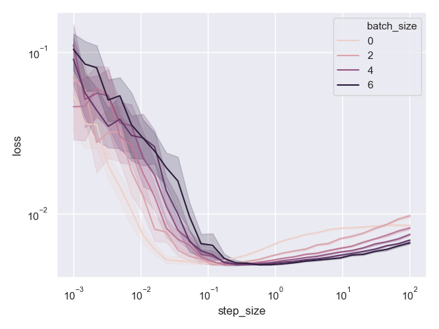
Seaborn’s hue coding is a bit confusing, since we don’t really have a batch size of 0, but it is clear that darker is higher. We can see that for small enough step sizes the method does not perform well. It is not surprising - taking small steps leads to slow convergence, and we are going to need much more than 10 epochs to converge. However, for a large range of step sizes beginning at approximately \(0.1\), the performance of the method is quite stable. Even for step sizes as large as \(10^2\), the method does not diverge!
Moreover, we clearly see that mini-batches improve the performance whenever we do converge to something plausible. Let’s plot the same data, but focused to step sizes at-least \(0.1\).
focused_losses = best_losses[best_losses['step_size'] >= 0.1]
sns.set()
ax = sns.lineplot(x='step_size', y='loss', hue='batch_size', data=focused_losses, err_style='band')
ax.set_yscale('log')
ax.set_xscale('log')
plt.show()
Here is the resulting plot:
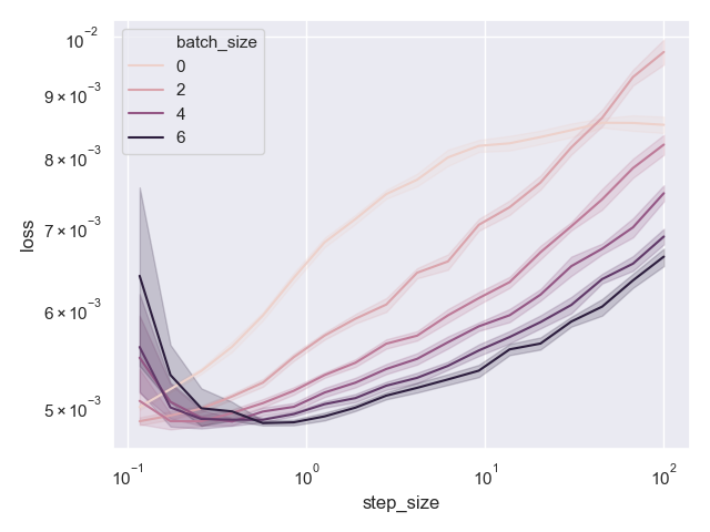
Indeed, darker colors, which correspond go higher batch sizes, lead to generally better results.
Teaser
Implementing a mini-batch version of the stochastic proximal point method poses a real challenge. This time, instead of solving simple one-dimensional optimization problems in each iteration we need to work harder, and solve \(\vert B \vert\) dimensional optimization problems. But we are seeing an interesting pattern - solving a large-scale optimization problem using a stochastic algorithm is done by solving a sequence of very small-scale classical optimization problems.
Consequently, we are going to talk about methods for solving the classical optimization problems which involve maximizing \(q(s)\) we derived in this post. Using the above, we will be able to build mini-batch optimizers for a variety of convex-on-linear losses. Stay tuned!