Review

In the previous post of this series, we introduced the stochastic proximal point (SPP) method for minimizing the average loss $\frac{1}{n} \sum_{i=1}^n f_i(x),$ according to which, at each step we choose $f \in \{f_1, \dots, f_n\}$ and step-size $\eta$, and compute

\[x_{t+1} = \operatorname*{argmin}_{x} \left\{ H_t(x) \equiv \color{blue}{f(x)} + \frac{1}{2\eta} \color{red}{\| x - x_t\|_2^2} \right\}.\]

Namely, the next iterate balances between minimizing $f$ and staying in close proximity to the previou siterate $x_t$. The optimizer implementing SPP must intimately know $f$, intimately enough so that it is able to solve the above problem and compute $x_{t+1}$. This ‘white box’ approach is in direct contrast to the standard ‘black box’ approach of SGD-type methods, where the optimizer sees $f$ through an oracle which is able to compute gradients.

The major challenge is in actually computing $x_{t+1}$, since the loss $f$ can be arbitrarily complex. Having paid the above price, the advantage obtained from stochastic proximal point is stability w.r.t the step-size choices, as demonstrated in the previous post.

This time

In this post we attempt to add some gray color to the white box, namely, we partially decouple some of the intimate knowledge about the loss $f$ from the SPP optimizer for a useful family of loss functions, which are of the form

\[f(x) = \phi(a^T x+b),\]

where $\phi$ is a one-dimensional convex function. The family above includes two important machine learning problems - linear least squares, and logistic regression. For linear least squares each loss is of the form $f(x)=\frac{1}{2} (a^T x + b)^2$, meaning that we have $\phi(t)=\frac{1}{2}t^2$, while for logistic regression each loss is of the form $\ln(1+\exp(a^T x))$¹, meaning that we have $\phi(t)=\ln(1+\exp(t))$.

We will first develop the mathematical machinery for dealing with such losses, and then we will implement and test an optimizer based on PyTorch.

The naive attempt

Consider the logistic regression setup. The loss functions are of the form

\[f(x)=\ln(1+\exp(a^Tx))\]

Writing explicitly, the SPP step is

\[x_{t+1}=\operatorname*{argmin}_x \left\{ M(x)\equiv \ln(1+\exp(a^T x))+\frac{1}{2\eta}\|x-x_t\|_2^2 \right\}.\]

Let’s try to compute $x_{t+1}$ `naively’ by solving the equation $\nabla M(x)=0$:

\[\nabla M(x)=\frac{\exp(a^T x)}{1+\exp(a^T x)} a + \frac{1}{\eta}(x-x_t)=0\]

Whoa! How do we solve such an equation? Personally, I am not aware of any explicit formula for solving the above equation. We can, of course, try numerical methods, but then we defeat the entire idea of using the proximal point method when we have simple formula for computing $x_{t+1}$ given $x_t$.

What gets us to the promised land is the powerful convex duality theory.

A taste of convex duality

Consider the problem minimization problem

\[\min_{x,t} \qquad \phi(t)+g(x) \qquad \text{s.t.} \qquad t = a^T x + b \tag{P}\]

Suppose problem (P) above has a finite optimal value $v(P)$. Let’s take a look at the following function:

\[q(s)=\inf_{x,t} \{ \phi(t)+g(x)+s(a^T x+b-t) \}\]

Instead of the constraint $t=a^T x + b$, we define an unconstrained optimization problem parameterized by a ‘price’ $s \in \mathbb{R}$ for violating the constraint. Why is $q(s)$ interesting? Because of the following careful, but simple observation:

\[\begin{align} q(s) &= \inf_{x,t} \{ \phi(t)+g(x)+s(a^T x+b-t) \} \\ &\leq \inf_{x,t} \{ \phi(t)+g(x)+s(a^T x+b-t) : t = a^T x + b \} \\ &= \inf_{x,t} \{ \phi(t)+g(x) : t = a^T x + b \} = v(\mathrm{P}) \end{align}\]

The above inequality holds since minimizing over the entire space produces a smaller value than minimizing over a subset. The observation above means that $q(s)$ is a lower bound on the optimal value of our desired problem (P). The dual problem is about finding the “best” lower bound:

\[\max_s \quad q(s). \tag{D}\]

This “best” lower bound $v(D)$ is still a lower bound - this simple property is called the weak duality theorem. But we are interested in the stronger result - strong duality:

Suppose that both $\phi(t)$ and g(x) are closed convex functions² and $v(P)$ is finite. Then,

(a) the dual problem (D) has an optimal solution $s^*$, and $v(P)=v(D)$, that is, the ‘best’ lower bound is tight.

(b) Moreover, if the minimization problem which is used to define $q(s^*)$ has a unique optimal solution $x^*$, then $x^*$ is the unique optimal solution of (P). Meaning, we can extract the optimal solution of (P) from the optimal solution of (D).

What we described above is a tiny fraction of convex duality theory, but this tiny fraction is enough for our purposes.

Why is it useful? Note that the dual problem we obtained is a one dimensional optimization problem. It can be as simple as maximizing a parabola!

Coloring the white box in gray

Now, let’s use convex duality. Assuming $f(x)=\phi(a^T x + b)$ , at each step we aim to compute

\[x_{t+1} = \operatorname*{argmin}_{x} \left\{ \phi(a^T x + b) + \frac{1}{2\eta} \| x - x_t\|_2^2\right\}.\]

Seems that the above proble has no constraints, but constructing a dual problem requires a constraint. So let’s add one! We define an auxiliaty variable $t=a^T x + b$, and obtain following equivalent formulation:

\[x_{t+1} = \operatorname*{argmin}_{x,t} \left\{ \phi(t) + \frac{1}{2\eta} \|x - x_t\|_2^2 : t = a^T x+b \right\}.\]

Let’s compute the dual problem:

\[\begin{aligned} q(s) &=\min_{x,t} \left \{ \phi(t) + \frac{1}{2\eta} \|x - x_t\|_2^2 + s(a^T x + b - t) \right \} \\ &= \color{blue}{\min_x \left \{ \frac{1}{2\eta} \|x - x_t\|_2^2 + s a^T x \right \} } + \color{red}{\min_t\{\phi(t)-st\}} + s b, \end{aligned}\]

where the second equality follows from seperability³. Note, that the blue part does not depend on $\phi$, and can be easily computed by equating the gradient of the term inside $\min$ with zero, since it is a strictly convex function of $x$. The resulting minimizer is

\[x=x_t-\eta s a, \tag{*}\]

and therefore, the blue term is:

\[\frac{1}{2\eta} \|(x_t - \eta s a) - x_t\|_2^2 + s a^T (x_t - \eta s a)=-\frac{\eta \|a\|_2^2}{2}s^2+(a^T x_t) s\]

The red part does depend on $\phi$, and can be alternatively written as

\[-\underbrace{\max_t \{ ts - \phi(t) \}}_{\phi^*(s)}.\]

The function $\phi^{*}(s)$ is well known in convex analysis, and is called the convex conjugate of $\phi$. One important property of $\phi^*$ is that it is always convex. Here are some well-known examples:

$\phi(t)$	$\phi^{*}(s)$
$\frac{1}{2}t^2$	$\frac{1}{2}s^2$
$\ln(1+\exp(t))$	$s \ln(s)+(1-s) \ln(1-s)$ where $0 \log(0) \equiv 0$
$-\ln(x)$	$-(1+\ln(-s))$

Summing up what we discovered about the red and blue parts, we obtained

\[q(s)=-\frac{\eta \|a\|_2^2}{2} s^2+(a^T x_t+b) s-\phi^*(s)\]

Having solved the dual problem of maximizing $q(s)$, conclusion (b) of the strong duality theorem says that we can obtain $x_{t+1}$ from the formula (∗). Thus, to compute $x_{t+1}$ we need to perform the following steps:

Compute the coefficients of $q(s)$, namely, compute $\alpha=\eta \|a\|_2^2$, and $\beta=a^T x_t + b$.
Solve the dual problem: find $s^{*}$ which maximizes $q(s)=-\frac{\alpha}{2}s^2 + \beta s - \phi^*(s)$
Compute: $x_{t+1}=x_t - \eta s^* a$.

Steps (1) and (3) do not depend on $\phi$, and can be performed by a generic optimizer, while step (2) has to be provided by the optimizer’s user, who intimately knows $\phi$.

Example 1 - Linear least squares

We consider $\phi(t)=\frac{1}{2} t^2$. According to the conjugate table above, we have $\phi^{*}(s)=\frac{1}{2}s^2$. The dual problem aims to maximize

\[q(s)=-\frac{\eta \|a\|_2^2}{2} s^2+(a^T x_t+b) s - \frac{1}{2}s^2=-\frac{\eta \|a\|_2^2+1}{2} s^2+(a^T x_t+b) s\]

Our $q(s)$ is a concave parabola, which is very simple to maximize. Its maximum is obtained at $s^*=\frac{a^T x_t+b}{1+\eta \|a\|_2^2}$, and thus the SPP step is

\[x_{t+1}=x_t-\frac{\eta (a^T x_t+b)}{1+\eta \|a\|_2^2}a\]

Magic! That is exactly the formula we obtained by tedious math in our previous post. No tedious math this time!

Example 2 - Logistic Regression

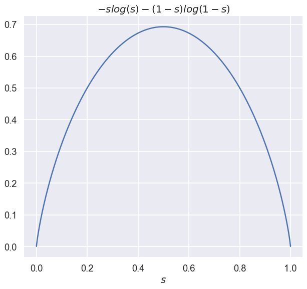
For logistic regression we define $\phi(t)=\log(1+\exp(t))$, and therefore $\phi^{*}(s)=s \log(s)+(1-s) \log(1-s)$, with the convention that $0 \log(0)\equiv 0$. The corresponding dual problem aims to maximize

\[\begin{aligned} q(s) &=-\frac{\eta \|a\|_2^2}{2} s^2+(a^T x_t+b) s-s \log(s)-(1-s)\log(1-s) \\ &=\color{magenta}{-\frac{\alpha}{2}s^2 + \beta s} -s \log(s)-(1-s)\log(1-s) \end{aligned}\]

Now, let’s analyze $q(s)$ a bit. First, note that because of the logarithms it is defined on the interval $[-1,1]$, and undefined elsewhere. It makes things a bit easier - we have to look for the maximizer in that interval only. Second, it is not hard to prove that it has a unique maximizer inside the open interval $(0,1)$, but such rigorous analysis is not the aim of this blog post, and we will do the convincing using a simple plot:

logistic_reg_conjugate

So now comes the interesting part - how do we find this maximizer? Well, let’s equate $q’(s)$ with zero:

\[q'(s)=-\alpha s + \beta+\log(1-s)-\log(s)=0\]

Seems like a hard equation to solve, but we are at luck. Concave functions have a decreasing derivative, and since $q’(s)$ is also continuous we can employ the bisection method, which is very similar to the well-known binary search:

\[\begin{aligned} &\textbf{Input:}~\mbox{continuous function $g$, interval $[l,u]$, tolerance $\mu > 0$} \\ &\textbf{Output:}~ x \in [l,u] \mbox{ such that }g(x) = 0 \\ &\textbf{Assumption:}~ \operatorname{sign}(g(l)) \neq \operatorname{sign}(g(u)) \\ &\textbf{Steps:} \\ & \quad \textbf{while} ~ u-l > \mu \text{:} \\ & \qquad m = (u + l) / 2 \\ & \qquad \textbf{if}~ g(m) = 0\text{:} \\ & \qquad \quad \textbf{return}~ m \\ & \qquad \textbf{if}~ \operatorname{sign}(g(m)) = \operatorname{sign}(g(l)) \text{:} \\ & \qquad \quad l = m \\ & \qquad \textbf{else} \text{:} \\ & \qquad \quad u = m \end{aligned}\]

The only challenge left is finding the initial interval $[l,u]$ where the solution lies, because we can’t use $[0,1]$ since $q’$ is undefined at its endpoints . But carefully looking at $q’(s)$ we conclude that when we approach $s=0$ it tends to infinity, while as we approach $s=1$ it tends to negative infinity. Thus, we can find $[l,u]$ using the following simple method:

$l=2^{-k}$ for the smallest positive integer $k$ such that $q’(2^{-k}) > 0$.
$u=1-2^{-k}$ for the smallest positive integer $k$ such that $q’(1-2^{-k}) < 0$.

Let’s code

Let’s begin by implementing our SPP solver for losses of the form $f(x)=\phi(a^T x + b)$. Recall our decoupling of the SPP step into ‘generic’ and ‘concrete’ parts. Let’s begin by implementing the generic part of the solver:

import torch

class ConvexOnLinearSPP:
    def __init__(self, x, eta, phi):
        self._eta = eta
        self._phi = phi
        self._x = x
        
    def step(self, a, b):
        """
        Performs the optimizer's step, and returns the loss incurred.
        """
        eta = self._eta
        phi = self._phi
        x = self._x
        
        # compute the dual problem's coefficients
        alpha = eta * torch.sum(a**2)
        beta = torch.dot(a, x) + b
        
        # solve the dual problem
        s_star = phi.solve_dual(alpha.item(), beta.item())
        
        # update x
        x.sub_(eta * s_star * a)
        
        return phi.eval(beta.item())
    
    def x(self):
        return self._x
        

Next, let’s implement our two $\phi$ variants:

import torch
import math

# 0.5 * t^2
class SquaredSPPLoss:
    def solve_dual(self, alpha, beta):
        return beta / (1 + alpha)
    
    def eval(self, beta):
        return 0.5 * (beta ** 2)
    
    
# log(1+exp(t))
class LogisticSPPLoss:
    def solve_dual(self, alpha, beta):
        def qprime(s):
            -alpha * s + beta + math.log(1-s) - math.log(s)
        
        # compute [l,u] containing a point with zero qprime
        l = 0.5
        while qprime(l) <= 0:
            l /= 2
        
        u = 0.5
        while qprime(1 - u) >= 0:
            u /= 2
        u = 1 - u
        
        while u - l > 1E-16: # should be accurate enough
            mid = (u + l) / 2
            if qprime(mid) == 0:
                return mid
            if qprime(l) * qprime(mid) > 0:
                l = mid
            else:
                u = mid
        
        return (u + l) / 2
   
    def eval(self, beta):
        return math.log(1+math.exp(beta))

Experiment

Let’s see if we observe the the same stability w.r.t the step-size choice for a logistic regression problem, similarly to what we saw for linear least squares in the previous post. We will use the Adult income dataset, whose purpose is predicting wheather income exceeds $50k/y based on census data. Full code can be found in this git repo.

This time I checked only one competitor - AdaGrad, since my computational resources are limited. But you are welcome to clone the repository, and check additional algorithms. Each algorithm ran 10 times for 20 epochs, and the best training loss of each run was recorded. Below are the results:

results

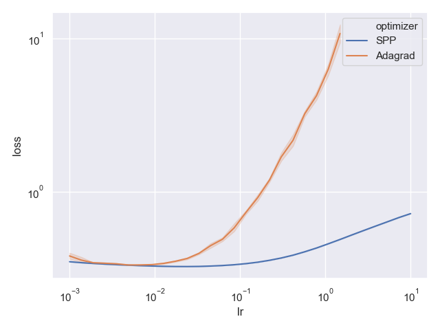
The x-axis is the step size, while the y-axis is the best achieved loss for that step-size among the epochs. It is not a surprise that this time as well we observe the same stability phenomenon: AdaGrad performs well for a narrow range of step-sizes, while the SPP method performs well for a very wide range of step-size choices, namely, it is less sensitive to the choice of step-sizes.

Teaser

In many machine learning problems, we don’t wish to merely solve a simple least squares or a logistic regression problem, but a regularized problem. For example, L2 regularized logistic regression aims to solve an average of losses of the form

\[f(x)=\log(1+\exp(a^T x)) + \alpha \|x\|_2^2\]

We will discuss regularization in the next post. Stay tuned!

The prediction of logistic regression $\hat{y} = 1/(1+\exp(-w^T x))$ for input $w$ composed with the log-loss $-y \ln(\hat{y})+ (1-y) \ln(1-\hat{y})$ for binary labels $y \in \{0,1\}$, after some algebra, results in $\ln(1+\exp(\pm w^T x))$. Defining $a = w$ or $a = -w$, depending on our sample’s label, results in losses of the form $\ln(1+\exp(a^T x))$. ↩
A function is closed if its epigraph $\operatorname{epi}(f)=\{ (x, y): y \geq f(x) \}$ is a closed set. Most functions of interest are closed, including the functions in this post. ↩
Separable minimization: $\min_{z,w} \{ f(z)+g(w) \} = \min_u f(z) + \min_v g(w).$ ↩

\(\phi(t)\)	\(\phi^{*}(s)\)
\(\frac{1}{2}t^2\)	\(\frac{1}{2}s^2\)
\(\ln(1+\exp(t))\)	\(s \ln(s)+(1-s) \ln(1-s)\) where \(0 \log(0) \equiv 0\)
\(-\ln(x)\)	\(-(1+\ln(-s))\)