“Selective approximation - the prox-linear method for training arbitrary models"
This post is part of the series "Proximal point", and is not self-contained.
Series posts:
-
“Proximal Point - warmup"
-
“Proximal point - convex on linear losses"
-
“Proximal Point - regularized convex on linear I"
-
“Proximal Point - regularized convex on linear II"
-
“Proximal Point is, after all, yet another gradient method"
- “Selective approximation - the prox-linear method for training arbitrary models" (this post)
-
“Proximal Point with Mini Batches"
-
“Proximal Point with Mini Batches - Convex On Linear"
-
“Proximal Point with Mini Batches - Regularized Convex On Linear"
-
“Proximal Point to the Extreme - Factorization Machines"
- “Proximal Point - warmup"
- “Proximal point - convex on linear losses"
- “Proximal Point - regularized convex on linear I"
- “Proximal Point - regularized convex on linear II"
- “Proximal Point is, after all, yet another gradient method"
- “Selective approximation - the prox-linear method for training arbitrary models" (this post)
- “Proximal Point with Mini Batches"
- “Proximal Point with Mini Batches - Convex On Linear"
- “Proximal Point with Mini Batches - Regularized Convex On Linear"
- “Proximal Point to the Extreme - Factorization Machines"
The proximal point approach which we explored in the last series of posts is an extreme approach - avoid any loss approximation, and work with it directly. But this extreme approach works only for a small subset of losses for which it is practical. The most general subset we explored was the regularized convex-on-linear. On the scale between using losses exactly on the one side and performing a full linear approximation, such as SGD, on the other side, there is diverse set of possibilities which rely on partial approximations. Carefully chosing which part we approximate and which we treat directly leads to practically implementable algorithms that can optimize a variety functions, while still enjoying some of the benefits of the proximal point approach. In this post we discuss one of them - the prox-linear method.
Our setup is minimizing the average loss of the form
\[\frac{1}{n} \sum_{i=1}^n \bigl[ \underbrace{\phi(g_i(x)) + r(x)}_{f_i(x)} \bigr],\]where \(\phi\) is a one-dimensional convex function, \(g_1, \dots, g_n\) are continuously differentiable, and the regularizer \(r\) is convex as well. Let’s take a minute to grasp the formula in the machine learning context: each of the functions \(g_i\) produces some affinity score of the \(i^{\text{th}}\) training sample with respect to the parameters \(x\), and the result is fed to \(\phi\) which produces the final loss, which is regularized with \(r\).
Before seeing some examples of why such decomposition of the losses into the inner parts \(g_i\) and the outer part \(\phi\) is useful, one remark is in place. Note, that since \(g_i\) can be an arbitrary function, we are dealing with a non-convex optimization problem, meaning that usually any hope of finding an optimum is lost. However, the practice of machine learning shows us that more often than not, stochastic optimization methods do produce reasonable solutions.
Examples
The first example is an arbitrary model with the L2 (mean squared error) loss for a regression problem. Namely, we have the training set \(\{ (w_i, \ell_i) \}_{i=1}^n\) with arbitrary labels \(\ell_i \in \mathbb{R}\), and we are training a model \(\sigma(w, x)\) which predicts the label of input \(w\) given parameters \(x\) by minimizing
\[\frac{1}{n} \sum_{i=1}^n \Bigl[ \tfrac{1}{2} \bigl( \underbrace{\sigma(w_i, x) - \ell_i}_{g_i(x)} \bigr)^2 + r(x) \Bigr].\]In this case, we have the outer loss \(\phi(t)=\tfrac{1}{2}t^2\). The model \(\sigma\) can be arbitrarily complex, i.e. a neural network or a factorization machine.
The second is an arbitrary model with the logistic loss. Namely, we have the training set \(\{(w_i, \ell_i)\}_{i=1}^n\) with binary labels \(\ell_i \in \{0,1\}\). We are training a model \(\sigma(w, x)\) whose prediction on input \(w\) given parameters \(x\) is the sigmoid
\[p(w,x)= \frac{1}{1+e^{-\sigma(w,x)}},\]which is trained by minimizing the regularized cross-entropy losses
\[\frac{1}{n} \sum_{i=1}^n \Bigl[ -\ell_i \ln(p(w_i, x)) - (1 - \ell_i) \ln(1 - p(w_i, x)) + r(x) \Bigr].\]At first glance the above formula does not appear to fall into our framework, but after some algebraic manipulation we can transform it into
\[\frac{1}{n} \sum_{i=1}^n \Bigl[\ln(1+\exp(\underbrace{(1-2\ell_i) \sigma(w_i, x)}_{g_i(x)})) + r(x) \Bigr].\]In this case, we have the convex outer loss \(\phi(t)=\ln(1+\exp(t))\). The model \(\sigma\) can be, again, arbitrarily complex.
Many other training setups fall into this framework, including training with the hinge loss, the mean absolute deviation, and many more. Note, that \(\phi\) does not even have to be differentiable.
The prox-linear approach
SGD-type methods eliminate the complexity imposed by arbitrary loss functions by using their linear approximations. We discuss a similar approach: eliminate the complexity imposed by arbitrary functions \(g_i\) by approximating them using a tangent. However, we keep the regularizer and the outer-loss intact, without approximating them. Conretely, at each iteration we select \(g \in \{ g_1, \dots, g_n \}\) and compute:
\[x_{t+1} =\operatorname*{argmin}_x \Biggl\{ \phi(\underbrace{g(x_t)+ \nabla g(x_t)^T( x - x_t) }_{\text{Linear approx. of } g(x)}) + r(x) + \frac{1}{2\eta} \|x - x_t\|_2^2 \Biggr\}.\]The partial approximation idea is not new, and in the non-stochastic setup dates back to the Gauss-Netwon algorithm from 1809. The stochastic setup, which is what we are dealing with in this post, has been recently analyzed in several papers12, and surprisingly has been shown to enjoy, under some technical assumptions, the same step-size stability properties we observed for proximal point approach provided that \(\phi\) is bounded below. For the two prototypical examples at the beginning of this post \(\phi\) is indeed bounded below: \(\phi(t) \geq 0\) for both of them. The boundedness property holds almost ubiquitously in machine learning.
In our approximation above, the term inside \(\phi\) is linear in \(x\), and can be explicitly re-written as
\[x_{t+1} = \operatorname*{argmin}_x \Biggl\{ \phi(\underbrace{\nabla g(x_t)}_a \ ^T x + \underbrace{g(x_t) - \nabla g(x_t)^T x_t}_b) + r(x) + \frac{1}{2\eta} \|x - x_t\|_2^2 \Biggr\}, \tag{PL}\]which falls exactly to the regularized convex-on-linear framework. For the above problem we already devised an efficient algorithm for computing \(x_{t+1}\), and wrote a Python implementation. The algorithm we devised relies on the proximal operator of the regularizer \(\operatorname{prox}_{\eta r}\), and on the convex conjugate of the outer loss \(\phi^*\). It consists of the following steps, with \(a\) and \(b\) taken from equation (PL) above:
- Solve the dual problem - find a solution \(s^*\) of the equation: \(a^T \operatorname{prox}_{\eta r}(x_t - \eta s a) + b - {\phi^*}’(s)=0\)
- Compute: \(x_{t+1} = \operatorname{prox}_{\eta r}(x_t - \eta s^* a)\)
Intuition and discussion
Before diving into an implementation, let’s take a short break to appreciate the method from an intuitive standpoint. In the last post we saw, visually, that the proximal point algorithm takes a step which differs from SGD both in its direction and its length. Let’s see what does the prox-linear method do.
For simplicity, imagine we have no regularization. In that case, step (2) in the algorithm above becomes
\[x_{t+1} = x_t - \eta s^* \nabla g(x_t)\]If we used SGD instead, it would be
\[x_{t+1} = x_t - \eta \ \phi’(g(x_t)) \nabla g(x_t)\]Looks similar? Well, it seems that the prox-linear differs from SGD only in the step’s length, but not in its direction - both go in the direction of \(\nabla g(x_t)\). Personally, I would be surprised if it would not be the case. We are relying on a linear approximation of \(g\), so it is only natural that the step is in the direction dictated by its gradient.
From a high-level perspective the prox-linear method adapts a step length to each training sample, but make no attempt to learn from the history of the training samples to adapt a step-size to each coordinate. In contrast, methods such as AdaGrad, Adam, and others of similar nature, adapt a custom step-size to each coordinate based on the entire training history, but make no attempt to adapt to each training sample separately. These two seem like two orthogonal concerns, and it might be interesting if they can somehow be combined to construct an even better optimizer.
A discussion about adapting a step length to each iteration of the optimizer is not complete without recalling another famous approach - the Polyak step-size3. It has nice convergence properties for deterministic convex optimization, and a variant has been recently analyzed in the stochastic machine-learning centric setting in a paper by Loizou et. al.4.
An optimizer for L2 regularization
Since it is simple to handle and widely used, let’s implement the algorithm for \(L2\) regularization \(r(x)=\frac{\alpha}{2} \|x\|_2^2\). Recalling that \(\operatorname{prox}_{\eta r}(u) = \frac{1}{1+\eta \alpha} u\), the algorithm amounts to:
- Solve the dual problem - find a solution \(s^*\) of the equation: \(\underbrace{g(x_t) - \frac{\eta \alpha \nabla g(x_t)^T x_t}{1+\eta \alpha}}_{c} - \underbrace{\frac{\eta \| \nabla g(x_t)\|_2^2}{1+\eta \alpha}}_{d} s - {\phi^*}'(s) = 0\)
- Compute: \(x_{t+1} = \frac{1}{1+\eta \alpha}(x_t - \eta s^* \nabla g(x_t))\)
Looking at the second step, some machine learning practitioners may recognize a variant of the well-known weight decay idea - the algorithm decays the parameters of the model by the factor \(1 + \eta \alpha\), after performing something that seems like a gradient step.
The first step in the algorithm above depends on the outer loss \(\phi\), while the second step can be performed by a generic optimizer. Since we need some machinery to compute of \(\nabla g_i\), we will implement the generic component as a full-fledged PyTorch optimizer and rely on the autograd mechanism built into PyTorch to compute \(\nabla g_i\).
import torch

class ProxLinearL2Optimizer(torch.optim.Optimizer):
    def __init__(self, params, step_size, alpha, outer):
        if not 0 <= step_size:
            raise ValueError(f"Invalid step size: {step_size}")
        if not 0 <= alpha:
            raise ValueError(f"Invalid regularization coefficient: {alpha}")

        defaults = dict(step_size = step_size, alpha = alpha)
        super(ProxLinearL2Optimizer, self).__init__(params, defaults)

        self._outer = outer

    def step(self, inner):
        inner_val = inner() # g(x_t)

        outer = self._outer
        loss_noreg = outer.eval(inner_val) # phi(g(x_t))

        # compute the coefficients (c, d) of the dual problem, and the regularization term
        c = inner_val
        d = 0
        for group in self.param_groups:
            eta = group['step_size']
            alpha = group['alpha']
            for p in group['params']:
                if p.grad is None:
                    continue

                c -= eta * alpha * torch.sum(p.data * p.grad).item() / (1 + eta * alpha)
                d += eta * torch.sum(p.grad * p.grad).item() / (1 + eta * alpha)

        # solve the dual problem
        s_star = outer.solve_dual(d, c)

        # update the parameters, and compute the regularization term.
        for group in self.param_groups:
            eta = group['step_size']
            alpha = group['alpha']
            for p in group['params']:
                if p.grad is None:
                    continue

                p.data.sub_(eta * s_star * p.grad)
                p.data.div_(1 + eta * alpha)

        # return the loss without regularization terms, like other PyTorch optimizers do, so that we can compare them.
        return loss_noreg
We could ada[t] the optimizer above to supporting sparse tensors, and add special handling to the case of no regularization, namely, \(\alpha = 0\), but for a blog-post it is enough. We can now train any model we like using our optimizer with a variant of the standard PyTorch training loop, for example:
model = create_model() # this is the model "sigma" from the beginning of this post
optimizer = ProxLinearL2Optimizer(mode.parameters(), learning_rate, reg_coef, SomeOuterLoss())

for input, target in data_set
    def closure():
        pred = model(input)
        inner = inner_loss(pred, target) # this is g_i
        inner.backward() # this computes the gradient of g_i
        return inner.item()

    opt.step(closure)
For our two prototypical scenarios we have already implemented the outer losses in previous posts, so I will just repeat them below for completeness:
import torch
import math

# 0.5 * t^2
class SquaredSPPLoss:
    def solve_dual(self, d, c):
        return c / (1 + d)

    def eval(self, inner):
        return 0.5 * (inner ** 2)


# log(1+exp(t))
class LogisticSPPLoss:
    def solve_dual(self, d, c):
        def qprime(s):
            -d * s + c + math.log(1-s) - math.log(s)

        # compute [l,u] containing a point with zero qprime
        l = 0.5
        while qprime(l) <= 0:
            l /= 2

        u = 0.5
        while qprime(1 - u) >= 0:
            u /= 2
        u = 1 - u

        while u - l > 1E-16: # should be accurate enough
            mid = (u + l) / 2
            if qprime(mid) == 0:
                return mid
            if qprime(l) * qprime(mid) > 0:
                l = mid
            else:
                u = mid

        return (u + l) / 2

    def eval(self, inner):
        return math.log(1+math.exp(inner))
Experiment
Model and setup
Let’s see how our optimizer does for training a factorization machine. I will be using the results of my collegue’s, Yoni Gottesman, phenomenal tutorial Movie Recommender from Pytorch to Elasticsearch, where he trains a factorization machine on the MovieLens 1M data-set to create a movie recommendation engine. He also shared a Jupyter notebook with the code. Readers unfamiliar with factorization machines are encouraged to read this, or any other tutorial, since I assume a basic understanding of the concept and its PyTorch implementation.
Since my focus is on optimization, e.g. training a model, I will assume that we have done all the data-preparation, and we have the table created Yoni’s notebook in a file called data_set.csv.
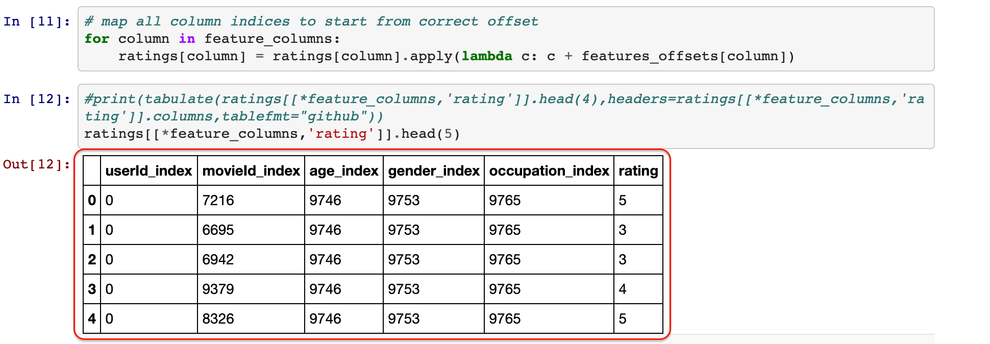
Each feature value is associated with an index, and \(m\) is the total number of distinct feature values.
We will be using a second-order factorization machine \(\sigma(w, x)\) for our recommendation prediction task. The model \(\sigma(w, x)\) is given a binary input \(w \in \{0, 1\}^m\) which encodes the feature values of the training sample, its parameter vector is \(x = (b_0, b_1, \dots, b_m, v_1, \dots, v_m)\) which is composed of the model’s bias \(b_0 \in \mathbb{R}\), the feature value biases \(b_1, \dots, b_m\in \mathbb{R}\), and the feature value latent vectors \(v_1, \dots, v_m \in \mathbb{R}^k\), where \(k\) is our embedding dimension. The model computes:
\[\sigma(w, x) := b_0 + \sum_{i = 1}^m w_i b_i + \sum_{i = 1}^m\sum_{j = i + 1}^{m} (v_i^T v_j) w_i w_j\]As the embedding dimension \(k\) increases, the model has more parameters to represent the data. Here is a PyTorch implementation of the model above, adapted from Yoni’s blog:
import torch
from torch import nn

def trunc_normal_(x, mean=0., std=1.):
    "Truncated normal initialization."
    # From https://discuss.pytorch.org/t/implementing-truncated-normal-initializer/4778/12
    return x.normal_().fmod_(2).mul_(std).add_(mean)

class FMModel(nn.Module):
    def __init__(self, m, k):
        super().__init__()

        self.b0 = nn.Parameter(torch.zeros(1))
        self.bias = nn.Embedding(m, 1)       # b_1, \dots, b_m
        self.embeddings = nn.Embedding(m, k) # v_1, \dots, v_m

        # See https://arxiv.org/abs/1711.09160
        with torch.no_grad():
            trunc_normal_(self.embeddings.weight, std=0.01)
        with torch.no_grad():
            trunc_normal_(self.bias.weight, std=0.01)

    def forward(self, w):
        # Fast impl. of pairwise interactions. See lemma 3.1 from paper:
        #    Steffen Rendle. Factorization Machines. In ICDM, 2010.
        emb = self.embeddings(w) # tensor of size (1, num_input_features, embed_dim)
        pow_of_sum = emb.sum(dim=1).pow(2)
        sum_of_pow = emb.pow(2).sum(dim=1)
        pairwise = 0.5 * (pow_of_sum - sum_of_pow).sum(dim=1)

        bias_emb = self.bias(w) # tensor of size (1, num_input_features, 1)
        bias = bias_emb.sum(dim=1)

        return self.b0 + bias.squeeze() + pairwise.squeeze()
Let’s try to train our model using the L2 loss. To save computational resources for this small example, I am going to train the model with embedding dimension \(k=8\) using and only for 5 epochs. Since I rely on the stability properties of the prox-linear optimizer, I chose the step_size arbitrarily.
import pandas as pd
import torch
from tqdm import tqdm

# create a Dataset object
df = pd.read_csv('dataset.csv')
inputs = torch.tensor(df[['userId_index','movieId_index','age_index','gender_index','occupation_index']].values)
labels = torch.tensor(df['rating'].values).float()
dataset = torch.utils.data.TensorDataset(inputs, labels)

# create the model
model = FMModel(m=inputs.max() + 1, k=8)

# run five training epochs
opt = ProxLinearL2Optimizer(model.parameters(), step_size=0.1, alpha=1E-5, outer=SquaredSPPLoss())
for epoch in range(5):
    train_loss = 0.
    for w, l in tqdm(torch.utils.data.DataLoader(dataset, shuffle=True)):
        opt.zero_grad()
        def closure():
            pred = model(w)
            inner = pred - l
            inner.backward()
            return inner.item()
        train_loss += opt.step(closure)

    print(f'epoch = {epoch}, loss = {train_loss / len(dataset)}')
I got the following output, discarding the tqdm progress bars:
epoch = 0, loss = 0.5289862413141884
epoch = 1, loss = 0.5224190998653859
epoch = 2, loss = 0.5189374542805951
epoch = 3, loss = 0.5175283396570431
epoch = 4, loss = 0.5169355024401286
Note that our loss is half of the mean squared error, so to get RMSE (root mean-squared error) we need to multiply it by two, and take the square root. The last epoch corresponds roughly to training RMSE of \(\approx 1.02\), which seems reasonable for a low-dimensional model of \(k=8\) and a guessed step-size which was not tuned in any way.
Stability experiment
Now, let’s do a more serious experiment which will test the stability of our optimizer w.r.t the step size choices, and compare it to AdaGrad. As in our first post, we will train our model with various step-sizes, for each step-size we will perform two experiments, and each experiment trains the model for 10 epochs and take the training loss from the best epoch. The multiple experiments exist to take into account the stochastic nature of training sample selection. Then, we will plot a graph of the average regularized5 training loss achieved for each step-size among the multiple experiments. The code is derived from what we have above.
import numpy as np
import pandas as pd
import torch
from tqdm import tqdm
import seaborn as sns

# create a Dataset object
df = pd.read_csv('dataset.csv')
inputs = torch.tensor(df[['userId_index','movieId_index','age_index','gender_index','occupation_index']].values)
labels = torch.tensor(df['rating'].values).float()
dataset = torch.utils.data.TensorDataset(inputs, labels)

# setup experiment parameters and results
epochs = range(10)
step_sizes = np.geomspace(0.001, 100, num=10)
experiments = range(0, 3)
exp_results = pd.DataFrame(columns=['optimizer', 'step_size', 'experiment', 'epoch', 'loss'])

# run prox-linear experiment
for step_size in step_sizes:
    for experiment in experiments:
        model = FMModel(m=inputs.max() + 1, k=8)
        opt = ProxLinearL2Optimizer(model.parameters(), step_size=step_size, alpha=alpha, outer=SquaredSPPLoss())
        for epoch in epochs:
            train_loss = 0.
            train_loss_reg = 0.
            desc = f'ProxLinear: step_size = {step_size}, experiment = {experiment}, epoch = {epoch}'
            for idx in tqdm(sampler, desc=desc):
                w, l = dataset[idx]
                opt.zero_grad()
                def closure():
                    inner = model(w) - l
                    inner.backward()
                    return inner.item()
                loss = opt.step(closure)
                train_loss += loss
                train_loss_reg += (loss + alpha * model.params_l2().item())

            train_loss /= len(dataset)
            train_loss_reg /= len(dataset)
            print(f'train_loss = {train_loss}, train_loss_reg = {train_loss_reg}')

            exp_results = exp_results.append(pd.DataFrame.from_dict(
                        {'optimizer': 'prox-linear',
                         'step_size': step_size,
                         'experiment': experiment,
                         'epoch': epoch,
                         'loss': [train_loss_reg]}), sort=True)

# run ada-grad experiment
for step_size in step_sizes:
    for experiment in experiments:
        model = FMModel(m=inputs.max() + 1, k=8)
        opt = torch.optim.Adagrad(model.parameters(), lr=step_size, weight_decay=alpha)
        for epoch in epochs:
            train_loss = 0.
            train_loss_reg = 0.
            desc = f'Adagrad: step_size = {step_size}, experiment = {experiment}, epoch = {epoch}'
            for idx in tqdm(sampler, desc=desc):
                w, l = dataset[idx]
                opt.zero_grad()
                def closure():
                    loss = 0.5 * ((model(w) - l) ** 2)
                    loss.backward()
                    return loss.item()
                loss = opt.step(closure)
                train_loss += loss
                train_loss_reg += (loss + alpha * model.params_l2().item())

            train_loss /= len(dataset)
            train_loss_reg /= len(dataset)
            print(f'train_loss = {train_loss}, train_loss_reg = {train_loss_reg}')

            exp_results = exp_results.append(pd.DataFrame.from_dict(
                        {'optimizer': 'Adagrad',
                         'step_size': step_size,
                         'experiment': experiment,
                         'epoch': epoch,
                         'loss': [train_loss_reg]}), sort=True)

# display the results
best_results = exp_results[['optimizer', 'step_size', 'experiment', 'loss']].groupby(['optimizer', 'step_size', 'experiment'], as_index=False).min()
sns.set()
ax = sns.lineplot(x='step_size', y='loss', hue='optimizer', data=best_results, err_style='band')
ax.set_yscale('log')
ax.set_xscale('log')
plt.show()
And after a few days we obtain the following result:
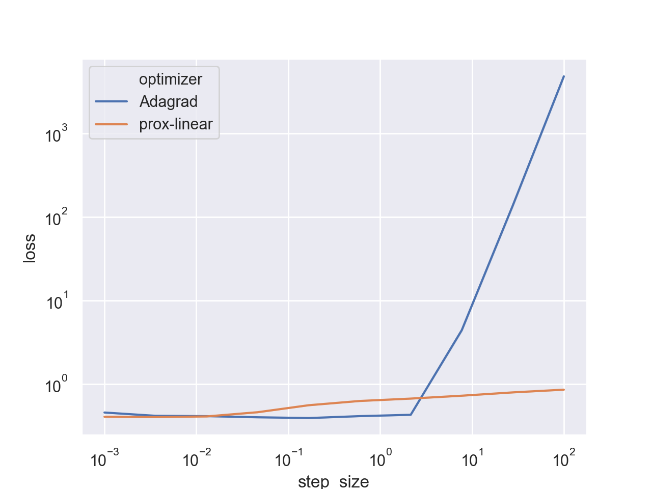
Seems that the algorithm is indeed stable, and does not diverge even when taking extremely large step sizes. However, AdaGrad does achieve a better loss for its optimal step-size range. To see a better picture, let’s focus on a smaller step size range:
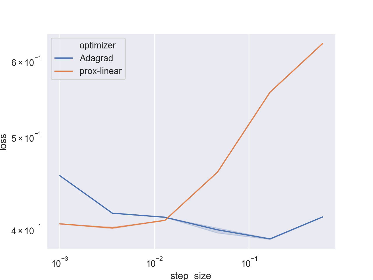
Seems that at this smaller range both algorithms seem stable, and AdaGrad even performs better. It is not surprising - we already saw that when using L2 regularization, AdaGrad tends to perform quite well. Let’s compare convergence rates for the optimal step sizes of each algorithm:
# extract convergence rate of each optimizer at its own optimal step size
convrate_pl = exp_results[(exp_results['step_size'] == 0.003593813663804626) & (exp_results['optimizer'] == 'prox-linear')].drop(['step_size'], axis=1)
convrate_adagrad = exp_results[(exp_results['step_size'] == 0.1668100537200059) & (exp_results['optimizer'] == 'Adagrad')].drop(['step_size'], axis=1)
convrate = convrate_pl.append(convrate_adagrad)

# plot the results
sns.lineplot(x='epoch', y='loss', hue='optimizer', data=convrate)
plt.show()
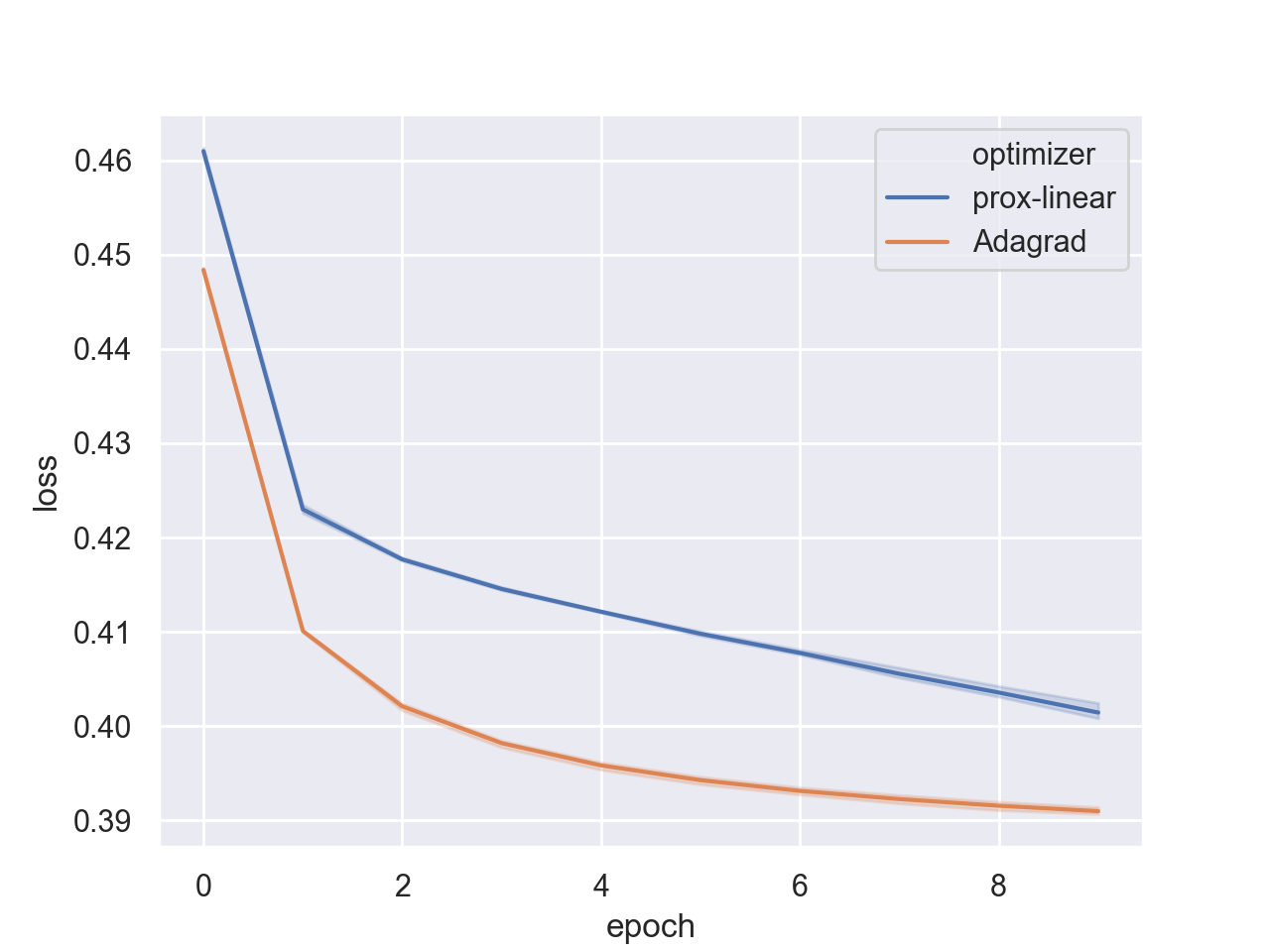
Indeed, the rate of AdaGrad’s convergence is substantially better. Seems that adapting a step size to each coordinate is more beneficial than adapting a step size to each training sample via the prox-linear algorithm. But we also saw that this approach really shines when the regularization is not L2, and we can actually benefit from not approximating the regularizer.
Despite its drawbacks, it’s still a reasonable algorithm to use when we don’t have the resources to tune the step size, but to get good results we will have to use more epochs to let it converge to a better solution. But our journey is not done - we will improve our optimizers using the framework we develop and see where it gets us.
Truncated loss approximations
For simplicity, suppose that we have no regularization (\(r=0\)). An interesting approach suggested in the paper1 by Asi & Duchi is using trunaced approximations for losses which are lower bounded, namely, \(f_i \geq 0\). Luckily, most losses in machine learning are lower bounded, and we can replace each \(f_i\) with
\[\max(0, f_i(x)),\]and treat \(\phi(t)=\max(0, t)\) as the outer loss and the original loss \(f_i\) as the inner loss. The computational step of the prox-linear method using the above inner/outer decomposition for \(f \in \{f_1, \dots, f_n\}\) becomes:
\[x_{t+1} = \operatorname*{argmin}_x \left\{ \max(0, f(x_t) + \nabla f(x_t)^T (x - x_t)) + \frac{1}{2\eta} \|x - x_t\|_2^2 \right\}.\]The above formula differs from regular SGD only in the fact that the linear approximation of \(f\) is trunaced at zero when it becomes negative, and is based on the simple intuition: if the loss is bounded below at zero, we shouldn’t allow its approixmation to be unbounded.
Remarkably, the above simple idea was proven by Asi & Duchi to enjoy similar stability properties, when the only information about the loss we exploit is the fact that it has a lower bound. By following the convex-on-linear solution recipe, we obtain an explicit formula for computing \(x_{t+1}\):
\[x_{t+1} = x_t - \min\left(\eta, \frac{f(x_t)}{\|\nabla f(x_t) \|_2^2} \right) \nabla f(x_t).\]That is, when the ratio of \(f(x_t)\) to the squared norm of the gradient \(\nabla f(x_t)\) is small, we take a regular SGD step of size \(\eta\). Otherwise, we modify the step length to be the above ratio. The above remarkably simple formula is enough to substantially improve the stability properties of SGD, both in theory and practice. The reason for not dealing with the above approach in this blog post, is because Hilal Asi, one of the authors of the above-mentioned paper1, already provided truncated approximation optimizers for both PyTorch and TensorFlow in this GitHub repo.
Teaser
The convex-on-linear framework has proven to be powerful enough to allow us to efficiently train arbitrary models using the prox-linear algorithm when taking individual training samples. Each training sample can be thought of as an approximation of the entire average loss, but the error of this approximation can be quite large. A standard practice to reduce this error is to use a mini-batch of training samples. In the next post we will discuss an efficient implementation for a mini-batch of convex-on-linear functions. Then, we will be able to derive a more generic prox-linear optimizer which can train arbitrary models using mini-batches of training samples.
Footnotes and references
-
Asi, H. & Duchi J. (2019). Stochastic (Approximate) Proximal Point Methods: Convergence, Optimality, and Adaptivity SIAM Journal on Optimization 29(3) (pp. 2257–2290) ↩ ↩2 ↩3
-
Davis, D. & Drusvyatskiy. D. (2019) Stochastic Model-Based Minimization of Weakly Convex Functions. SIAM Journal on Optimization 29(1) (pp. 207-239) ↩
-
Polyak B. T. (1987) Introduction to Optimization. Optimization and Software, Inc., New York ↩
-
Loizou N. & Vaswani S. & Laradji I. & Lacoste-Julien S. (2020) Stochastic Polyak Step-size for SGD: An Adaptive Learning Rate for Fast Convergence. Arxiv preprint: https://arxiv.org/abs/2002.10542 ↩
-
We use a regularized loss, since we are minimizing the regularized loss, and would like to appreciate the performance of optimizers as optimizers. The choice of the regularization parameter which achieves a good validation loss has to be done using standard techniques in machine learning. We may be able to avoid extensive step size tuning, but we still have to find the optimal regularization coefficient. ↩